
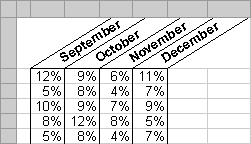
Rotate text and borders The data in a column is often very narrow while the label for the column is much wider. Instead of creating unnecessarily wide columns or abbreviated labels, you can rotate text and apply borders that are rotated to the same degree as the text.
Add borders, colors, and patterns To distinguish between different types of information in a worksheet, you can apply borders to cells, shade cells with a background color, or shade cells with a color pattern.
You can use number formats to change the appearance of numbers, including dates and times, without changing the number behind the appearance. The number format does not affect the actual cell value that Microsoft Excel uses to perform calculations. The actual value is displayed in the formula bar.
The General number format
The General format is the default number format. For the most part, numbers formatted with the General format are displayed just the way you entered them. However, if the cell is not wide enough to show the entire number, the General format rounds numbers with decimals and uses scientific notation for large numbers.
Built-in number formats
Excel contains many built-in number formats you can choose from. To list them, click Cells on the Format menu, and then click the Number tab. The Special category includes formats for postal codes and phone numbers. Options for each category appear to the right of the Category list. The formats appear in categories on the left, including Accounting, Date, Time, Fraction, Scientific, and Text.
Apply an autoformat to a range or list To format an entire list or other range that has distinct elements
Create and apply a style To apply several formats in one step and ensure that cells have consistent formatting, you can apply a style to the cells. Microsoft Excel has styles you can use to format numbers as currency, as percentages, or with commas that separate thousands. You can create your own styles to apply a font and font size, number formats, cell borders, and shading and to protect cells from changes. If your data is in an outline, you can apply styles according to outline level.
Copy formats from one cell or range to another If you've already formatted some cells on a worksheet the way you want, you can use the Format Painter button to copy the formatting to other cells.
Automatically extend formats When this option is on, the formatting is automatically extended when you enter rows at the end of a range that you've already formatted. You can turn automatic formatting on or off.
 Formatting cells based on specific conditions
You can monitor formula results or other cell values by applying conditional formats. For example, you can apply green text color to the cell if sales exceed forecast and red shading if sales fall short.
When conditions change If the value of the cell changes and no longer meets the specified condition, Microsoft Excel clears the formatting from the cell, but leaves the condition applied so that the formatting will be automatically reapplied when the condition is met.
Shared workbooks In a shared workbook, conditional formats that are applied before a workbook is shared continue to work; however, you cannot modify the conditional formats or apply new ones while the workbook is shared.
PivotTable reports If you try to apply conditional formats to cells in a PivotTable report, you will get unpredictable results.
Formulas as formatting criteria
You can compare the values of the selected cells to a constant or to the results of a formula. To evaluate data in cells outside the selected range or to examine multiple sets of criteria, you can use a logical formula to specify the formatting criteria.
- Use the value in a cell as the condition If you select the Cell Value Is option and compare the values of the selected cells to the result of a formula, you must start the formula with an equal sign (=).
- Use a formula as the condition If you select the Formula Is option, the formula you specify must return a logical value of TRUE (1) or FALSE (0). You must start the formula with an equal sign (=). The formula can evaluate data only on the active worksheet. To evaluate data on another sheet or in another workbook, you can define a name on the active worksheet for the data on another sheet or workbook, or enter a reference to the data in a cell of the active worksheet. Then refer to that cell or name in the formula. For example, to evaluate data in cell A5 on Sheet1 of the workbook Fiscal Year.xls, enter the following reference, including the equal sign (=), in a cell of the active sheet: =[Fiscal Year.xls]SHEET1!$A$5
The formula can also evaluate criteria that is not based on worksheet data. For example, the formula =WEEKDAY("12/5/99")=1 returns a value of TRUE if the date 12/5/99 is a Sunday. Unless a formula specifically refers to the selected cells you are formatting, the cell values do not affect whether the condition is true or false. If a formula does refer to the selected cells, you must enter the cell references in the formula.
- Use cell references as the condition You can enter cell references in a formula by selecting cells directly on a worksheet. Selecting cells on the sheet inserts absolute cell references. If you want Microsoft Excel to adjust the references for each cell in the selected range, use relative cell references.
- Use dates Dates and times are evaluated as serial numbers. For example, if you compare the cell value with the date January 7, 2001, the date is represented by the serial number 36898.
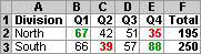
In the following example, conditional formats applied to the range B2:E3 analyze quarterly contributions to the yearly total. Quarterly results that contribute 30 percent or more to the total are displayed in bold and green. Quarterly results that contribute 20 percent or less are displayed in bold and red.
The following table summarizes the conditional formats applied to the range B2:E3. Microsoft Excel adjusts the relative portion (the row number) of the cell reference $F2 in the formula so that each cell in the range B2:E3 is compared with the corresponding total in column F.
| Cell Value Is | Formula | Formats | |
|---|---|---|---|
| Condition 1 | Greater than or equal to | =$F2*0.3 | Bold, green font |
| Condition 2 | Less than or equal to | =$F2*0.2 | Bold, red font |
Example 2: Use a formula and external cell references
| Formula Is | Formats | |
|---|---|---|
| Condition 1 | =AND(AVERAGE($A$1:$A$5)>3000, MIN($A$1:$A$5)>=1800) |
Green cell shading |
Example 3: Use a formula and a cell reference
| Formula Is | Formats | |
|---|---|---|
| Condition 1 | =MOD(A4,2)=0 | Blue font |
This formula must evaluate each cell in the range. When you enter such a formula in the Conditional Formatting dialog box, however, enter only the cell reference for the active cell in the selected range. Microsoft Excel adjusts the references to the other cells relative to the active cell.
Verify a conditional format before applying it An easy way to ensure that formula references are correct is to apply the conditional formatting first to one cell in the range. Then select the entire range, click Conditional Formatting on the Format menu, and then click OK. The conditional formatting you applied to the first cell is applied to the entire range, with the formula correctly adjusted for each cell.