Enables you to watch cells and their formulas on the Watch Window toolbar, even when the cells are out of view.
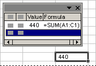
Watch Window
This toolbar can be moved or docked like any other toolbar. For example, you can dock it on the bottom of the window. The toolbar keeps track of the following properties of a cell: workbook, sheet, name, cell, value, and formula.
You can only have one watch per cell.
Like a grammar checker, Excel uses certain rules to check for problems in formulas. These rules do not guarantee that your spreadsheet is problem-free, but they can go a long way to finding common mistakes. You can turn these rules on or off individually.
Problems can be reviewed in two ways: one at a time like a spelling checker, or immediately on the worksheet as you work. A triangle appears in the top-left corner of the cell when a problem is found. Both methods present the same options.

Cell with a formula problem
A problem can be resolved using the options that appear, or it can be ignored. If a problem is ignored, it does not appear in further error checks. However, all previously ignored errors can be reset so that they appear again.
The rules and what they check for
Evaluates to error value The formula does not use the expected syntax, arguments, or data types. Error values include #DIV/0!, #N/A, #NAME?, #NULL!, #NUM!, #REF!, and #VALUE!. Each error value has different causes, and is resolved in different ways.
Note If you enter an error value directly in a cell, it is not marked as a problem.
Text date with 2 digit years The cell contains a text date that can be misinterpreted as the wrong century when used in formulas. For example, the date in the formula =YEAR("1/1/31") could be 1931 or 2031. Use this rule to check for ambiguous text dates.
Number stored as text The cell contains numbers stored as text. These usually come from data imported from other sources. Numbers stored as text can cause unexpected sorting behaviors, and it is best to convert them to numbers.
 Inconsistent formula in region
The formula does not match the pattern of other formulas near it. In many cases formulas that are adjacent to other formulas only differ in the references used. For example, the formula =SUM(A10:F10) would be noted because the adjacent formulas change by one row, and it changes by 8 rows.
| Formulas |
|---|
| =SUM(A1:F1) |
| =SUM(A2:F2) |
| =SUM(A10:F10) |
| =SUM(A4:F4) |
If the references used in a formula are not consistent with those in the adjacent formulas, then the problem is noted.
The formula may not include a correct reference. If a formula refers to a range of cells, and you add cells to the bottom or right of that range, the references may no longer be correct. The formula does not always automatically update its reference to include the new cells. This rule compares the reference in a formula against adjacent cells. If the adjacent cells contain more numbers (are not blank cells), then the problem is noted.
For example, the formula =SUM(A2:A4) would be noted with this rule, because A5, A6, and A7 are adjacent, and contain data.
| Invoice |
|---|
| 15,000 |
| 9,000 |
| 8,000 |
| 20,000 |
| 5,000 |
| 22,500 |
| =SUM(A2:A4) |
Unlocked cells contain formulas
The formula is not locked for protection. By default, all cells are locked for protection, so the cell has been set to be unprotected. When a formula is protected it cannot be modified without being unprotected. Check to make sure you do not want the cell protected. Protecting cells that contain formulas prevents them from being changed, and can help avoid future errors.
The formula contains a reference to an empty cell. This can cause unintended results, as in the following example.
Suppose you want to take the average of the numbers below. If the third cell down is blank, then the result is 22.75. If the third cell down contains 0, then the result is 18.2.
| Data |
|---|
| 24 |
| 12 |
| 45 |
| 10 |
| Formula |
|---|
| =AVERAGE(A2:A6) |
Use the Formula Auditing toolbar to graphically display, or trace, the relationships between cells and formulas with blue arrows. You can trace the precedents (the cells that provide data to a specific cell) or you can trace the dependents (the cells that depend on the value in a specific cell).
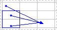
Worksheet with tracer arrows
You can see the different parts of a nested formula evaluated in the order the formula is calculated by using the Evaluate Formula dialog box (Formula Auditing toolbar). For example, you can see this in the following formula where the function AVERAGE(F2:F5) is shown as its value 80.
=IF(AVERAGE(F2:F5)>50,SUM(G2:G5),0) as
=IF(80>50,SUM(G2:G5),0)
Notes
- Some parts of formulas that use the IF and CHOOSE functions are not evaluated, and #N/A is displayed in the Evaluation box.
- If a reference is blank, a zero value (0) is displayed in the Evaluation box.
- The following functions are recalculated each time the worksheet changes, and can cause the Evaluate Formula to give results different from what appears in the cell. RAND, AREAS, INDEX, OFFSET, CELL, INDIRECT, ROWS, COLUMNS, NOW, TODAY, RANDBETWEEN.