Model Background
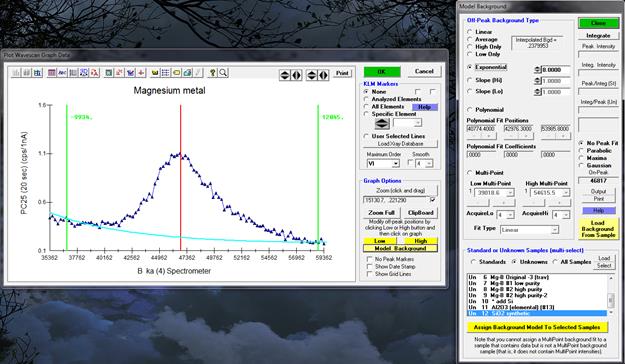
To model the various off-peak background correction types, click the Model Background button. This option is only available when a wavescan sample is displayed.
To see the background model, click the specific background type and observe the plotted background curve in the Graph window.
For the exponential, slope and polynomial off-peak background types coefficients are required. The exponential, slope-high and slope-low coefficients are entered by hand. The exponential exponent may be –6 to +6. For high or low only background types, a slope of one (1.) will produce exactly the same result as the high-only or low-only off-peak background type. In situations where there is some curvature and exponential cannot be used, examination of backgrounds on similar phases that lack the element of interest can give an appropriate "slope" factor to yield a proper background at the peak position. For example, if the high-only offset had a value of 10 and the slope factor entered was 1.3, the on peak background used would be 13.
The polynomial background fit coefficients are calculated automatically as the three different fit positions are moved by clicking the minus (-) or plus (+) buttons. The slope or polynomial coefficients can be applied to selected standard or unknown samples for use with a sample specific slope or polynomial off-peak background correction. That is, the actual slope or polynomial background correction will be calculated for each sample based on the actual off-peak data for that sample using the fit coefficients from the fit model.
To make the assignment to the selected unknown samples, be sure to click Ok in the Model Background dialog AND ALSO in the Graph Data dialog.
Calculating Specified or Compound APF Ratios
To calculate specified or binary Peak/Integrated and Integrated/Peak ratios for use with the specified or compound Area Peak Factor (APF) correction methods, one might be required to perform careful high precision wavescans and calculate the peak and integrated intensities of the analytical peak in question to correct for peak shift and/or shape changes. This is usually the case for new compounds or other binary systems where prior measurements by Bastin are not found in the literature.
The first point is that whether you will utilize the Peak/Integrated intensity or the Integrated/Peak intensity depends on whether this wavescan is the "std" material or the "unk" material for the APF calculation. That is, use the P/I ratio from your standard material wavescan (the same as the primary quant standard) and use the I/P ratio from your unknown material wavescan (the same as your unknown sample).
By using the Model Background dialog one can utilize the Integrate button to perform most of these intensity calculations quickly and easily. An example for Boron Ka in Mg compounds is provided.
But first an important consideration:
depending on whether you keep the peak position constant for the different
standard and unknown materials (and thereby incorporate the peak shift effect in
the APF calculation) or use a different peak position for each material (and
minimize the peak shift and essentially only correct for peak shape changes, in
addition to improving your counting statistics by using optimized peak
positions), how you go about calculating the APF is slightly different for the
two cases.
After loading a wavescan (on the standard or unknown
material) to be used for the APF calculation, into the Graph dialog, click the
Model Background button. If one now clicks the Integrate button the program
calculates the Peak and Integrated intensities and also the P/I and I/P
intensities based on the on-peak position of the wavescan sample. By default,
the Probe for EPMA program uses the peak position recorded for each wavescan
sample. Now if you are using the same peak position for all samples (and
correcting for both peak shift and peak shape changes) that is fine. Multiply
your P/I and I/P ratio from your two materials, edit your EMPAPF.DAT file and
you are done.
Now in the case of sulfur the change
between, say pyrite and anhydrite is almost all peak shift, so you probably
wouldn't want to use the same spectrometer position for both materials though
you could if you were consistently using the same peak position for both the
wavescans and the standard and unknown samples. Also if the spectral
change between the two materials is mostly peak shape them you probably would
also use the same spectrometer positions and just correct for changes in peak
shape.
But if you want to minimize the peak shift effect and use the
optimum peak position for each material (and optimize your counting statistics),
and only correct for peak shape changes, you should either make sure that each
wavescan has the correct on-peak position specified before acquisition. Or you
can click one of the peak fit options in the Model Background dialog (usually
Maxima or Highest). Then click the Integrate button again and the program will
recalculate the P/I and I/P values based on the newly fitted peak
position.
Of course you must use the same optimized peak positions for
your actual quantitative standard and unknown acquisitions if you use APFs based
on these fitted peak positions.
Multi-Point Backgrounds
Adjustment of multi-point backgrounds can also be performed graphically using the wavescan plot Model Background dialog. Select the High or Low side multi-point background and use the plus and minus buttons to graphically adjust the position on the wavescan. The number of background points on each side of the peak to acquire can also be specified here.
The number of points to iterate to and the background fit type (Linear or Polynomial) can be specified before or after the background intensity data has been acquired. Note that the sum of all multi-point intensities is automatically calculated and saved to the normal off-peak intensity arrays to so that normal off-peak background calculations can also be performed.