Calculate Detection Limits
The user may also select a calculation of the single point detection limits, single point percent analytical sensitivity, average homogeneity, average range of homogeneity, average detection sensitivity and average weight percent analytical sensitivity. The single point calculations are output for all data points, the sample average calculation are output only when the sample contains two or more data points and are expressed as t-test confidence intervals from .60 (60% confidence) to .99 (99% confidence). The t-test values will decrease detection limit and analytical sensitivity confidence significantly if only a few data points are acquired. Generally five to ten data points are necessary for a relatively robust confidence interval prediction.
Single Point Detection Limits:
The single point detection limit calculation is based on the standard counts and the unknown background counts and including the magnitude of the ZAF correction factor. The calculation is adapted from Love and Scott (1983). This detection limit calculation is useful in that it can be used even on inhomogeneous samples and can be quoted as the detection limit in weight percent for a single analysis line with a confidence of 99% (assumes 3 standard deviations above the background).
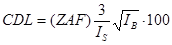
Where : ZAF is the ZAF correction factor for the sample matrix
 is the
count rate (cps/nA) on the (pure element) standard (apply std
k-factor)
is the
count rate (cps/nA) on the (pure element) standard (apply std
k-factor)
 is the
background count rate (cps/nA) on the unknown sample, see note below*
is the
background count rate (cps/nA) on the unknown sample, see note below*
*In the above calculation be aware that before calculating the SQRT of the background count rate, one must first de-normalize the count rate (cps/nA) to raw counts by noting the beam current and integration time for the unknown intensity. Then take the SQRT, and finally re-normalize the background intensity to cps/nA before calculating the above k-ratio IB/IS. A sample DebugMode output is shown here for examination:
Line: 144 Intermediate Detection Limits Calculations (nominal beam = 1):
Element/Xray ti ka fe ka al ka mn ka mg ka
Bgd Count/Sec 3.1 1.4 1.3 .3 .7
Bgd CountTime 1200.00 1200.00 1200.00 1200.00 1200.00
Bgd Beam Curr 100.10 100.10 100.10 100.10 100.10
Bgd Raw Count 369342. 171492. 154624. 37771.2 84664.8
Bgd Dev Raw 607.7 414.1 393.2 194.3 291.0
Bgd Dev Cps .005059 .003447 .003274 .001618 .002422
Std Count/Sec 1894.82 1019.25 331.900 164.413 979.149
Std K-Factor .5616 .6862 .1159 .4052 .4215
Std Cps @100% 3373.97 1485.35 2863.61 405.753 2322.84
Unk ZAF Corr 1.2627 1.1927 1.6733 1.2235 2.1261
Detection limit at 99 % Confidence in Elemental Weight Percent (Single Line):
ELEM: Ti Fe Al Mn Mg
144 .00057 .00083 .00057 .00146 .00067
Single Point Analytical Sensitivities:
After this, a rigorous calculation of analytical error also for single analysis lines is performed based on the peak and background count rates from both the unknown and the standard also from Love and Scott 1983. The results of the calculation are displayed after multiplication by a factor of 100 to give a percent analytical error of the net count rate. This analytical error result can be compared to the percent relative standard deviation (%RSD) displayed in the analytical calculation (both are one sigma standard deviation levels). The analytical error calculation is as follows:
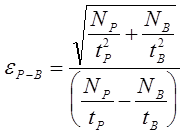
Where
:
 is the total
peak counts
is the total
peak counts
 is the total
background counts
is the total
background counts
 is the peak count time
 is the background count time
Note that the single point analytical sensitivity calculations utilize the interference, blank corrected, etc. on-peak intensities for the most accurate calculation.
Average Detection Limits and Analytical Sensitivity:
A more comprehensive set of calculations for analytical statistics is also performed on the averaged sample data if the sample contains two or more data points. These statistics are based on equations adapted from "Scanning Electron Microscopy and X-Ray Microanalysis" by Goldstein, et. al. (Plenum Press, 1992 ed., 1981) p. 432 - 436. All calculations are expressed for various confidence intervals from 60 to 99 % confidence.
Note that the average detection limit and analytical sensitivity calculations utilize the interference, blank corrected, etc. on-peak intensities for the most accurate calculation.
The calculations are based on the number of data points acquired in the sample and the measured average and standard deviation for each element. This is important because although x-ray counts theoretically have a standard deviation equal to square root of the mean, the actual standard deviation is usually larger due to variability of instrument drift, x-ray focusing errors, and x-ray production. The statistical calculations include :
The trace element detection limit is in elemental weight percent and indicates the minimum concentration detectability limit (CDL). Because this calculation utilizes the actual variance (standard deviation) of the measured composition, it should only be utilized for homogeneous materials.
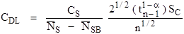
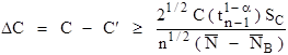
The analytical sensitivity is in elemental weight percent and indicates what a statistically significant difference between two concentrations is. Because this calculation utilizes the actual variance (standard deviation) of the measured composition, it should only be utilized for homogeneous materials.
Where
:
 is the
concentration to be compared with
is the
concentration to be compared with
C is the actual concentration in weight percent of the sample
Cs is the actual concentration in weight percent of the standard
 is the Student t
for a 1-α confidence and n-1 degrees of freedom
is the Student t
for a 1-α confidence and n-1 degrees of freedom
n is the number of data points acquired
 is the
standard deviation of the measured values (count intensity)
is the
standard deviation of the measured values (count intensity)
 is the average number of counts on the unknown
 is the
continuum background counts on the unknown
is the
continuum background counts on the unknown
 is the
average number of counts on the standard
is the
average number of counts on the standard
 is the continuum
background counts on the standard
is the continuum
background counts on the standard
The detection limit calculation here is intended only for use with homogenous samples since the calculation includes the actual standard deviation of the measured counts. This detection limit can, however, be quoted for the sample average and of course will improve as the number of data points acquired increases. The analytical sensitivity calculation is ignored for elements whose concentrations are present at less than 1%.
An option exists for the Projected Detection Limits in which the program extrapolates for shorter and longer count times how much of an effect changing the counting time will have on the detection limit. Based on the assumption that doubling the count time will decrease the detection limit by Sqr(2).