Home > Getting Started Guide > Creating a Simple Pivot Table in Excel > Pivot Tables Excel 2007 > Create a Pivot Table Report
Create a Pivot Table Report
To create a Pivot Table you need to identify these two elements in your data:
Have a list in Microsoft Excel with data fields (headings) and rows of related data
Identify which fields are going to go where in your design
Method
Select any cell in the data list.
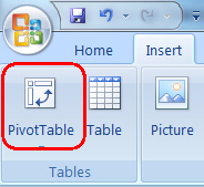
From the Insert tab, in the Tables group, click Pivot Table.
Make sure that Select a table or range is selected.
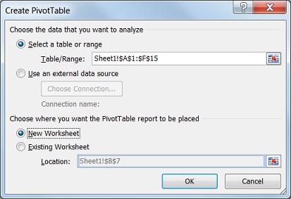
Make sure your data is listed in the Table/Range box.
Select where you want the Pivot Table to go, either in an Existing Worksheet or New Worksheet.
Click OK.
A blank Pivot Table will now be displayed.
![]()
In the Field List either select the fields you want in the Row Labels or drag them into the Row Labels area on the Field List box.
Repeat for Report Filter, Columns Labels and Values.