Analysing Single-channel Currents > Channel Dwell Time Analysis > Fitting exponential Functions to dwell time histograms
Dwell time distributions can usually be described in terms of a mixture of exponential probability density functions, where the probability p(t) of dwell time, t, being observed is given by
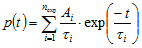
where nexp is the number of exponential components in the mixture, Ai is the fraction of the total number of dwell times associated with component i, and i is the mean dwell time. Mixtures of up to 5 exponential p.d.f.s can be to the dwell time histograms, using either an iterative least squares method.
Fitting Exponential Probability Density Functions
To fit an exponential mixture to a histogram:
1. Define the range of dwell times containing the histogram bins exponential distributions to be fitted using the pair of grey ‘|--|’ region of interest cursors. 
2. Select the number of exponential components in the mixture to be fitted from the Curve Fitting list.
3. Click the Fit Curve button and enter an appropriate set of initial guesses for the exponential function parameters (Ai, i). A set of initial guesses are computed automatically, but it is often necessary to adjust these to better match the location and size of the observed distribution. E.g. set the mean dwell times to the peaks in a logarithmic histogram.). Individual function parameters can also be fixed at their initial values by ticking its associated Fixed box. 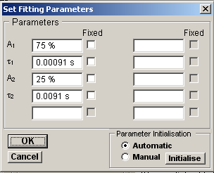
Click the OK button to begin fitting.
The mixture and the best fitting individual exponential components are superimposed (in red) on the histogram. The values of the function parameters along with their standard errors are displayed in curve fitting results area at the bottom of the display.
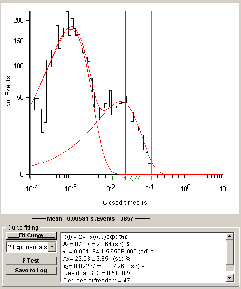
Note. Standard error values computed by the curve fitting program are not true estimates of experimental standard error since they take no account of inter-cell or other variability. They tend only provide a lower bound to the estimate of the standard error in a parameter value.) The residual standard deviation (SDres) between the histogram data and the fitted curve provides a measure of the goodness of fit. The smaller the value of SDres the better the fit.
Iterative curve fitting is a numerical approximation technique, which is not without its limitations. In some circumstances, it can fail to converge to a meaningful answer, in others the best fit parameters may be poorly defined. It is important to make an assessment of how well the function fits the histogram before placing too much reliance on the parameters.
Determining the required number of exponential components
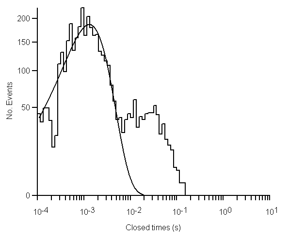
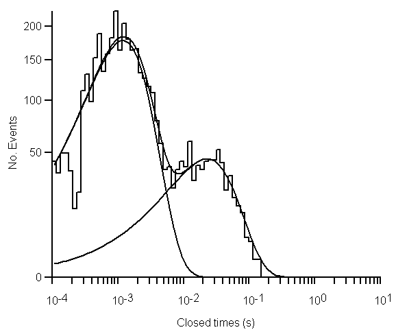
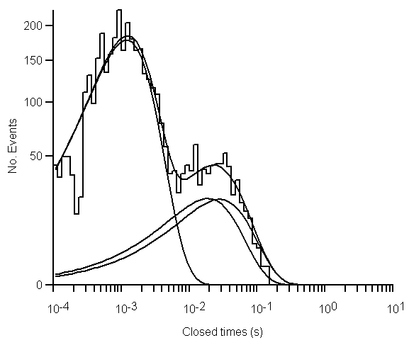
The number of components necessary to fit a dwell time distribution can be determined by fitting a series of exponential p.d.f. mixtures with increasing numbers of components, until no significant improvement in fit is observed. For example, the figures below show the results of fitting mixtures of 1, 2 and 3 exponential components.
The single exponential p.d.f. can be clearly seen to be a poor fit, with marked deviations between the fitted line and the data.
The mixture of two exponentials provides a qualitatively better fit, accounting for both peaks in the distribution. The residual standard deviation has also been reduced, indicating a better quantitative fit.
The mixture of three exponentials (c) also provides a qualitatively good fit, with a residual standard deviation similar to the two exponential fit. Two of the components appear to be very similar mean values
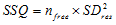
It is usual to choose the p.d.f. function with the least number of parameters, sufficient to provide a good fit. Additional components should only be included if they can be demonstrated to significantly improve the quality of fit. A quantitative estimate of the improvement in the quality of the fit, obtained by adding additional exponential components, can be obtained by computing the F statistic
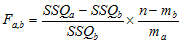
SSQa and SSQb are the sums of squares of the residual differences between the histogram data and the expected values for two p.d.f. functions a and b, where function a contains fewer exponential component than b. ma and ma are the number of free parameters in each function and n is the number of histogram bins. SSQ can be calculated for each function from the residual standard deviation, SDres and degrees of freedom, nfree, values returned as part of the curve fitting results.
Large positive values of Fa,b indicate that extra exponentials in function b result in a better fit to the data than function a, small positive values indicate that the fit is little improved and negative that it is worse. The significance probability of the observed Fa,b value can be determined from a standard F distribution, with ma and n – mb as its degrees of freedom. Further details can be found in Horn (1987).
To compare the quality of fit of the series of p.d.f.s fitted to a histogram, click the F Test button 
to open the F Test box.
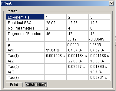
The residual sum of squares, number of function parameters and degrees of freedom for each function that has been fitted are tabulated.
For each successive exponential component the F statistic comparing its quality of fit with the previous one is computed along with its associated significance probability, p. A function is deemed to have significantly improved the quality of fit, if p <= 0.05. In the example shown here, 2 exponentials provide a significantly better fit (p=0.0000) than, but 3 exponentials do not provide a better fit than 2 (p=0.9805.)
Click the Print button to print a hard copy of the F test results table. The table of results can be cleared by clicking the Clear Table button.