Analysing Single-channel Currents > Channel Dwell Time Analysis > Plotting a Dwell Time Histogram
To plot a dwell time histogram:
1. Set the type of histogram to be plotted using the Histogram Type list.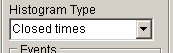
2. Select the All Events option to use all channel state events in the recording or select Range and enter the sub-range of events to be included.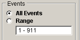
3. If Burst Length, or any of the other burst-related histogram types have been selected, enter the critical closed time value used to distinguish between intra- and inter-burst closed intervals in the T.critical box.
4.
5. Histogram Settings: Set the type of bin spacing to be used.Set the number of histogram bins in the No. Bins box.
Select the Linear option for fixed width bins and enter the lower and upper limits of the range of times to be included in the histogram in the Range box a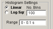
OR select the Log-Sqr option for logarithmically spaced bins and enter the number of bins per 10 fold change in dwell time in the No. bins per decade box.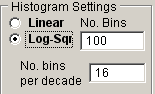
6. Click the New Histogram button to plot the histogram.
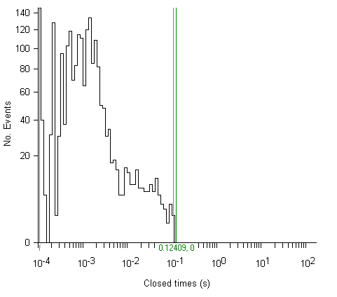
Linear histograms with fixed width bins
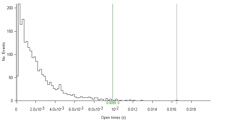
A Linear dwell time histogram is compiled by counting the number of state dwell times which fall into a series of equal sized time bins spread over a given range of times. Each dwell time, tstate, is assigned a bin number, ibin, according to the formula
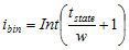
where w is the width of the bin, and Int means 'take the integer part of'. The exponential shape of the typical ion channel dwell time distribution is clearly apparent in a linear histogram.
Logarithmic histograms with variable bin widths
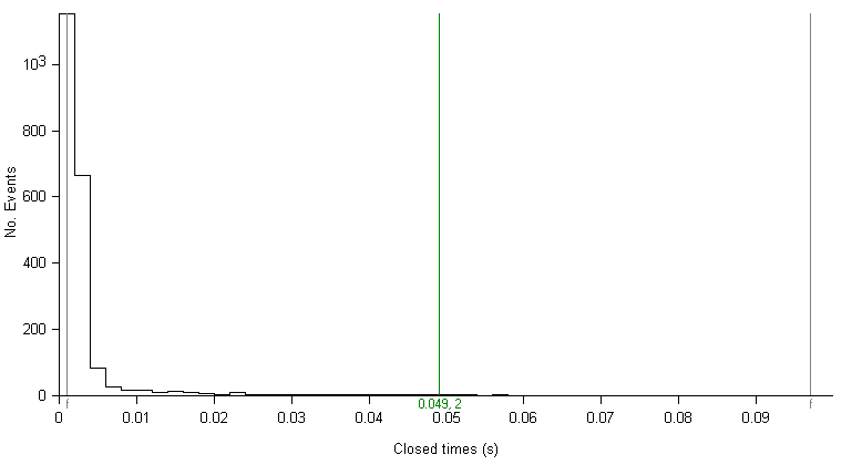
Many channels, however, produce open or closed distributions consisting of more than one type of state with radically different mean dwell times. In such circumstances it proves difficult to adequately represent the whole distribution of times using a single fixed bin width. For example, a closed time distribution composed of two types of states, one with a mean dwell time of 1 ms and the other with a mean of 40 ms cannot be easily represented on a linear histogram, as shown in the example histogram (100 bins, 1ms bin width). The 1ms bin width is too large to adequately represent the distribution of the short closures and too small to accumulate significant numbers of the long events in any one. bin.
One solution to the binning problems encountered with multi-state distributions is to begin with narrow bin widths for brief events and to progressively increase bin width for subsequent bins. An approach like this, developed by Sigworth & Sine (1987), has found widespread use. Dwell times are allocated to bins according to the formula
where bpd is the number of histogram bins per decade (10-fold) change in dwell time. and nd is the dwell time in units of sampling intervals. This algorithm results in a histogram consisting of a series of bins which logarithmically increase in width, from a bin size equal to the sampling interval, by the factor bpd every decade. By convention, the vertical axis of the Sigworth-Sine histogram is plotted using a square root scaling.
A typical logarithmic histogram is shown here (the same two-state, 1 ms, 40 ms closed time distribution used earlier). Each exponential now appears as a peaked distribution with the peak value occurring at the mean dwell time for that state.