Time Domain
Time Domain allows you to view a device response as a function of time. The following are discussed in this topic:
Note: Time Domain measurements are only available on analyzers with Option 010. See Configurations
See the updated App Note: Time Domain Analysis Using a Network Analyzer.
In normal operation, the analyzer measures the characteristics of a test device as a function of frequency. With Time Domain (opt 010), the frequency information is used to calculate the inverse Fourier transform and display measurements with time as the horizontal display axis. The response values appear separated in time, allowing a different perspective of the test device's performance and limitations.
The graphic below compares the same cable reflection measurement data in both the frequency and time domain. The cable has two bends. Each bend creates a mismatch or change in the line impedance.
The frequency domain S11 measurement shows reflections caused by mismatches in the cable. It is impossible to determine where the mismatches physically occur in the cable.
The time domain response shows both the location and the magnitude of each mismatch. The responses indicate that the second cable bend is the location of a significant mismatch. This mismatch can be gated out, allowing you to view the frequency domain response as if the mismatch were not present. Distance Markers can be used to pinpoint the distance of the mismatch from the reference plane.
How the Analyzer Measures in the Time Domain
Time domain transform mode simulates traditional Time-Domain Reflectometry (TDR), which launches an impulse or step signal into the test device and displays the reflected energy on the TDR screen. By analyzing the magnitude, duration, and shape of the reflected waveform, you can determine the nature of the impedance variation in the test device.
The analyzer does not launch an actual incident impulse or step. Instead, a Fourier Transform algorithm is used to calculate time information from the frequency measurements. The following shows how this occurs.
A single frequency in the time domain appears as a sine wave. In the following graphic, as we add the fundamental frequency (F0), the first harmonic (2F0), and then the second harmonic (3F0), we can see a pulse taking shape in the Sum waveform. If we were to add more frequency components, the pulse would become sharper and narrower. When the analyzer sends discrete frequencies to the test device, it is in effect, sending individual spectral pieces of a pulse separately to stimulate the test device.
During an S11 reflection measurement, these incident signals reflect from the test device and are measured at the A receiver. This is when the time domain transform calculations are used to add the separate spectral pieces together.
For example, consider a short length of cable terminated with an open. All of the power in the incident signal is reflected, and the reflections are 'in-phase' with the incident signal. Each frequency component is added together, and we see the same pattern as the simulated incident would have looked (above). The magnitude of the reflection is related to the impedance mismatch and the delay is proportional to the distance to the mismatch. The x-axis (time) scale is changed from the above graphic to better show the delay.
Alternately, the same cable terminated with a short also reflects all of the incident power, but with a phase shift of 180 degrees. As the frequency components from the reflection are added together, the sum appears as a negative impulse delayed in time.
For simplicity, we have discussed incident signals reflecting off discontinuities in the test device. By far the most common network analyzer measurement to transform to time domain is a ratioed S11 measurement. An S11 reflection measurement does not simply display the reflections measured at the A receiver - it displays the ratio (or difference) of the A receiver to the Reference receiver. In addition, the S11 measurement can also be calibrated to remove systematic errors from the ratioed measurement. This is critical in the time domain as the measurement plane, the point of calibration, becomes zero on the X-axis time scale. All time and distance data is presented in reference to this point. As a result, both magnitude and time data are calibrated and very accurate.
The following shows where the time domain transform occurs in the analyzer data flow: (see Data Access Map)
Acquire raw receiver (A and R1) data
Perform ratio (A/R1)
Apply calibration
Transform data to time domain
Display results
Therefore, although a time domain trace may be displayed, a calibration is always performed and applied to the frequency domain measurement which is not displayed.
The most common type of measurement to transform is an S11 reflection measurement. However, useful information can be gained about a test device from a transformed S21 transmission measurement. The frequency components pass through the test device and are measured at the B receiver. If there is more than one path through the device, they would appear as various pulses separated in time.
For example, the following transmission measurement shows multiple paths of travel within a Surface Acoustic Wave (SAW) filter. The largest pulse (close to zero time) represents the propagation time of the shortest path through the device. It may not be the largest pulse or represent the desired path. Each subsequent pulse represents another possible path from input to output.
Triple travel is a term used to describe the reflected signal off the output, reflected again off the input, then finally reappearing at the output. This is best seen in a time domain S21 measurement.
Measurement Response Resolution
In the previous paragraphs, we have seen that using more frequency components causes the assembled waveform to show more detail. This is known as measurement response resolution, which is defined as the ability to distinguish between two closely spaced responses.
Note: Adjusting the transform time settings improves display resolution, but not measurement resolution.
The following graphic shows the effect of both a narrow and wide frequency span on the response resolution. The wider frequency span enables the analyzer to resolve the two connectors into separate, distinct responses.
Resolution Formula
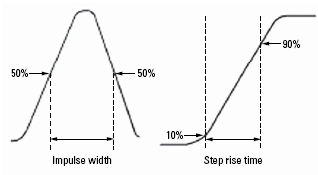
For responses of equal amplitude, the response resolution is equal to the 50% (−6 dB) points of the impulse width, or the step rise time which is defined as the 10 to 90% points as shown in the following image.
The following table shows the approximated relationship between the frequency span and the window selection on response resolution for responses of equal amplitude.
Window |
Low-pass step (10% to 90%) |
Low-pass impulse (50%) |
Bandpass impulse |
Minimum |
0.45 / f span |
0.60 / f span |
1.20 / f span |
Normal |
0.99 / f span |
0.98 / f span |
1.95 / f span |
Maximum |
1.48 / f span |
1.39 / f span |
2.77 / f span |
For example, using a 10 GHz wide frequency span and a normal window in Bandpass impulse mode, response resolution (in time) equals:
Time Res = 1.95 / frequency span
Time Res = 1.95 / 10 GHz
Time Res = 195 ps
To calculate the physical separation (in distance) of the responses which can be resolved, multiply this value times the speed of light (c) and the relative velocity (Vf) of propagation in the actual transmission medium. In this case, Vf = 0.66 for polyethylene dielectric.
Distance Res = 195 ps x c x Vf
Distance Res = 195 ps x (2.997925 E8 m/s) x .66
Distance Res = 38 mm
For reflection measurements, because of the 2-way travel time involved, this means that the minimum resolvable separation between discontinuities is half of this value or 19 mm.
Although a wider frequency span causes better measurement resolution, the measurement range becomes limited. Also, increasing the frequency range can cause a measurement calibration to become invalid. Be sure to adjust the frequency span BEFORE performing a calibration.
Measurement Range and Alias Responses
Measurement range is the length in time in which true time domain responses can be seen. The measurement range should be large enough to see the entire test device response without encountering a repetition (alias) of the response. An alias response can hide a true time domain response.
To increase measurement range in both modes, change either of these settings:
Increase the number of points
Decrease the frequency span
Notes:
After making these settings, you may need to adjust the transform time settings to see the new measurement range.
Decreasing the frequency span degrades measurement resolution.
Make frequency span and number of points settings BEFORE calibrating.
Maximum range also depends on loss through the test device. If the returning signal is too small to measure, the range is limited regardless of the frequency span.
Alias Responses
An alias response is not a true device response. An alias response repeats because each time domain waveform has many periods and repeats with time (see How the Analyzer Measures in the Time Domain). Alias responses occur at time intervals that are equal to 1/ frequency step size.
The analyzer adjusts the transform time settings so that you should only see one alias free range on either side (positive and negative) of zero time. However, these settings are updated only when one of the toolbar settings are changed.
To determine if a response is true, put a marker on the response and change the frequency span. A true device response will not move in time. An alias response will move.
For example, in the above graphic, the marker 1 response occurs at 14.07 inches. When the frequency span is changed, this response remains at 14.07 inches. The marker 2 response moves.
Range Formula
You can calculate the alias-free measurement range (in meters) of the analyzer using the following formula for TDR (reflection) measurements:
Range (meters) = (1/Δf) x Vf x c
Where:
Δf = frequency step size (frequency span/number of points-1)
Vf = the velocity factor in the transmission line
c = speed of light = 2.997925 E8 m/s
For example: For a measurement with 401 points and a span of 2.5 GHz, using a polyethylene cable (Vf = 0.66)
Range = (1 / (2.5E9 / 400)) x 2.997925 E8 m/s x 0.66
Range = 6.25E6 x 2.997925 E8 m/s x 0.66
Range = 32 meters
In this example, the range is 32 meters in physical length. To prevent the time domain responses from overlapping or aliasing, the test device must be 32 meters or less in physical length for a transmission measurement.
To calculate the one-way distance for a reflection measurement rather than round-trip distance, simply divide the length by 2. In this case, the alias-free range would be 16 meters.
How to make Time Domain SettingsThe following launches the Time Domain toolbar
On the toolbar, click More... to launch the Time Domain dialog box |
|
Using front-panel hardkey [softkey] buttons |
Using Menus |
|
|
|
|

Category Select Transform, Window, or Gating Transform Turns time domain transform ON and OFF. Coupling Settings Launches the Trace Coupling Settings dialog box. Time SettingsThe following settings adjust the display resolution, allowing you to zoom IN or OUT on a response. They do NOT adjust measurement range or measurement resolution. These settings automatically update (when one of these values are updated) to limit the display to one alias-free response on either side of zero time. Start Sets the transform start time that is displayed on the analyzer screen. Note: Zero (0) seconds is always the measurement reference plane. Negative values are useful if moving the reference plane. Stop Sets the transform stop time that is displayed on the analyzer screen. Center Sets the transform center time that is displayed in the center of the analyzer screen. Span Sets the transform span time that is split on either side of the Center value. Transform ModeTransform modes are three variations on how the time domain transform algorithm is applied to the frequency domain measurement. Each method has a unique application.
The following chart shows how to interpret results from various discontinuity impedances using Low pass Step and either Low pass or Band pass Impulse modes.
Effect on Measurement Range Band pass mode - measurement range is inversely proportional to frequency step size. Low pass mode - measurement range is inversely proportional to the fundamental (start ) frequency AFTER clicking Set Freq. Low Pass.
Set Freq. Low Pass USE ONLY IN LOW PASS MODES Recomputes the start frequency and step frequencies to be harmonics of the start frequency. Start frequency is computed by the following formula: Low Pass Start Frequency = Stop Frequency / Number of points. The computed value must always be greater than or equal to the analyzer's minimum frequency. Note: The number of points or stop frequency may be changed in order to compute this value. Distance Marker Settings Launches the Distance Marker Settings dialog box. |
Perhaps the most beneficial feature of time domain transform is the Gating function. When viewing the time domain response of a device, the gating function can be used to "virtually" remove undesired responses. You can then simultaneously view a frequency domain trace as if the undesired response did not exist.. This allows you to characterize devices without the effects of external devices such as connectors or adapters.
Note: When a discontinuity in a test device reflects energy, that energy will not reach subsequent discontinuities. This can "MASK", or hide, the true response which would have occurred if the previous discontinuity were not present. The analyzer Gating feature does NOT compensate for this.
The following measurements images show a practical example how to use and perform gating. The test device is a 10inch cable, then a 6 dB attenuator, terminated with a short. The following four discontinuities are evident in window 2, from left to right:
A discontinuity in the test system cable which appeared after calibration. It is identified by marker 2 at -10.74 inches (behind the reference plane).
A discontinuity in the 10 inch device cable shortly after the reference plane.
The largest discontinuity is the attenuator and short shown by marker 1 at -12.67 dB ( 6 dB loss in both forward and reverse direction).
The last discontinuity is a re-reflection from the device cable.
We will gate IN the attenuator response. All other responses will be gated OUT.
Window 1. Create original S11 frequency domain trace. Shows ripple from all of the reflections.
Window 2. Create a new S11 trace - same channel; new window. Turn Transform ON.
Window 3. On the transformed trace, turn gating ON. Center the gate on the large discontinuity (2.500ns). Adjust gate span to completely cover the discontinuity. Select Bandpass gating type.
Window 4. On the original frequency measurement, turn Gating ON (Transform remains OFF). View the measurement without the effects of the two unwanted discontinuities. The blue trace is a measurement of the 6 dB attenuator with the unwanted discontinuities PHYSICALLY removed. The difference between the two traces in window 4 is the effect of "masking".
Learn how to launch the Transform dialog box

Gating Turns Gating ON and OFF. Coupling Settings Launches the Setup Trace Coupling dialog box. Start Specifies the start time for the gate. Stop Specifies the stop time for the gate. Center Specifies the value at the center of the area that is affected by the gating function. This value can be anywhere in the analyzer range. Span Specifies the range to either side of the center value of area that is affected by the gating function. Gate Type Defines the type of filtering that will be performed for the gating function. The gate start and stop flags on the display point toward the part of the trace you want to keep.
Gate Shape Defines the filter characteristics of the gate function. Choose from Minimum, Normal, Wide, Maximum
Cutoff time -- is the time between the stop time (-6 dB on the filter skirt) and the peak of the first sidelobe. The diagram below shows the overall gate shape and lists the characteristics for each gate shape.
Minimum gate span -- is twice the cutoff time. Each gate shape has a minimum recommended gate span for proper operation. This is a consequence of the finite cutoff rate of the gate. If you specify a gate span that is smaller that the minimum span, the response will show the following effects:
|
There are abrupt transitions in a frequency domain measurement at the start and stop frequencies, causing overshoot and ringing in a time domain response. The window feature is helpful in lessening the abruptness of the frequency domain transitions. This causes you to make a tradeoff in the time domain response. Choose between the following:
Minimum Window = Better Response Resolution - the ability resolve between two closely spaced responses.
Maximum Window = Dynamic Range - the ability to measure low-level responses.
Learn how to launch the Transform dialog box
Coupling Settings Launches the Setup Trace Coupling dialog box. The window settings balance response resolution versus dynamic range.
The following three methods all the set window size. For best results, view the time domain response while making these settings.
Learn more about Windowing (top)
|
You can launch the Trace Coupling Settings dialog box from any of the following dialog boxes: |
|
Trace coupling allows you to change time domain parameters on a measurement, and have the same changes occur for all other measurements in the channel. For example: If you are simultaneously viewing a frequency domain measurement and time domain measurement, and Coupling is enabled in this dialog box, and ALL Gating Parameters are checked in this dialog box, and on the time domain measurement you change the Gate Span parameter, Then the frequency domain measurement will automatically change to reflect the time domain gated span. Note: Trace coupling applies ONLY to the Y-axis scale/reference settings. There are no changes to your data as a result of trace coupling. Coupling ON/OFF Check to enable coupling. All of the measurements in the active channel are coupled. The following parameters are available for coupling: Transform Parameters Stimulus Start, Stop, Center, and Span TIME settings. State (On/Off) Transform ON and OFF Window Kaiser Beta / Impulse Width Mode Low Pass Impulse, Low Pass Step, Band Pass Gating Parameters Stimulus Start, Stop, Center, and Span TIME settings. State (On/Off) Gating ON and OFF Shape Minimum, Normal, Wide, and Maximum Type Bandpass and Notch
|
To launch the Distance marker dialog box, click Dist. Marker Settings on the Transform dialog box.
When markers are present on a time domain measurement, distance is automatically displayed on the marker readout, marker table, and print copy. To learn how to create markers on your measurement see marker settings. You can read out impedance versus time by creating a marker on a Time Domain trace, then changing the marker format to R+jX. Learn how. This dialog box allows you to customize the time domain distance marker readings. These settings affect the display of ALL markers for only the ACTIVE measurement (unless Distance Marker Unit is coupled on the Trace Coupling dialog box. Marker Mode Specifies the measurement type in order to determine the correct marker distance.
Auto If the active measurement is an S-Parameter, automatically chooses reflection or transmission. If the active measurement is a non S-Parameter, reflection is chosen. Reflection Displays the distance from the source to the receiver and back divided by two (to compensate for the return trip.) Transmission Displays the distance from the source to the receiver. Units Specifies the unit of measure for the display of marker distance values. Velocity Factor Specifies the velocity factor that applies to the medium of the device that was inserted after the measurement calibration. The value for a polyethylene dielectric cable is 0.66 and 0.7 for PTFE dielectric. 1.0 corresponds to the speed of light in a vacuum. This is useful in Time Domain for accurate display of time and distance markers. This setting can also be made from the Electrical Delay and Port Extensions dialog boxes.
|