Synaptic Current Driving Function Analysis > Computing a Driving Function
The synaptic current driving function is a measure of the rate of evoked release of transmitter at a synapse. If the time course of decay the post-synaptic current is known, the driving function can be computed using a deconvolution process. More details of the method can be found in Dempster (1984). WinWCP’s driving function module can be used to compute the driving function from synaptic current records, such as endplate currents.
To carry out a driving function analysis:
a) Record a series of stimulus-evoked synaptic currents.
b) Use the signal averaging module to create an average synaptic current from the set of raw records.
c) Use the curve fitting module to fit an exponential function to the decay phase of the averaged synaptic current. Fit the function from around 95% - 5% of the decay phase, excluding the 5% around the peak where the transmitter is still being release.
d) Select
Analysis
Driving Function
to open the driving function window
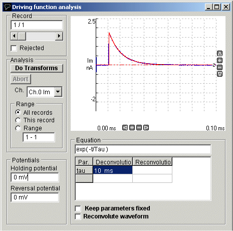
1) If there are several channels in the record, select the channel containing the signal to be transformed from the Ch. list.
2) Set the range of records to be transformed. Select All Records for all the records in the file, This Record for the currently displayed record only, or select Range and enter a range of records into the box.
3) Enter the cell holding potential (in mV) that the currents were recorded at, in the Holding Potential box, and the reversal potential of the post-synaptic current, in the Reversal Potential box. (The driving function is expressed in units of conductance/unit time. The holding and reversal potentials are required to convert from current to conductance).
4) The time constant computed by the curve fitting module in step (3) is used to deconvolve the current signal. If you wish to use the same time constant for all records (rather than using the individual value computed from each record), select the Keep parameters fixed option.
5) The basic deconvolution process computes a driving function, which represents the rate of change of post synaptic conductance induced by the release of transmitter. It is also possible to reconvolve this driving function with a different post-synaptic current decay function to generate the waveform of the synaptic current that would have existed under these new conditions. If you wish to create a simulated current, select the Reconvolute waveform option and enter the new time constant in the Reconvolution column.
6) Click the Do Transforms button to begin the deconvolution process.
Driving functions are created and stored in a driving function data file (.DFN extension) and can be viewed by selecting Driving Functions from the View menu to display them in the record display module.
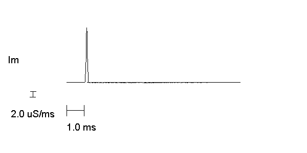
The driving function (b) computed from a simulated endplate current (a) is shown below.
(a)
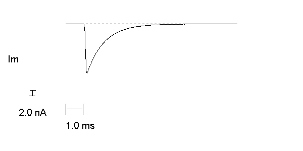
(b)