Fitting Gaussian Curves to Histograms
From WinWCP V5.3.8
Automatic Waveform Measurement > Fitting Gaussian Curves to Histograms
Gaussian probability density functions, representing the distribution of discrete populations of events, can be fitted to a histogram using non-linear least squares curve fitting. The number of events expected to be found in each histogram bin for a distribution represented by a mixture of m gaussians is given by
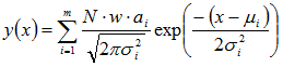
where N is the total number of events (records), w is the histogram bin width and each gaussian, i, is defined by three parameters, its mean, i, standard deviation, i and the fraction of the total number of events, ai, contained within it.
To fit a gaussian curve to the displayed histogram:
1) Select the number of gaussian functions (1, 2 or 3) to be fitted from the equations list. 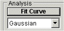
2) Define the region within the histogram to which the curve is to be fitted using the pair of vertical analysis region cursors. The selected region is indicated by the horizontal bar at the bottom of the display.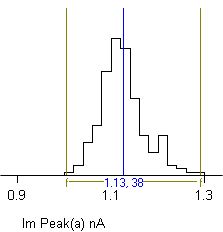
3) Click the Fit Curves button to start the curve fitting process. The initial parameter guesses are displayed in the Set Fitting Parameters dialog box. 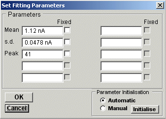
If you want to keep a parameter fixed (i.e. not changed by curve fitting process) tick its Fixed box. You can also change the initial parameter guesses, if they appear to be unrealistic. Click the OK button to fit the curve.
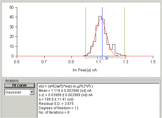
The best fitting curve is superimposed on the X/Y graph (in red) and the best fit equation parameters are displayed in the Curve Fitting table, along with the parameter standard error, the residual standard deviation (between the fitted and data points), statistical degrees of freedom in the fit, and the number of iterations it took to find the best fit.