Curve Fitting > Fitting Curves Signal Waveforms
Select
Analysis
Curve Fitting
to open the curve fitting window,
The module is split 5 functional sections (pages) – Curve Fitting, X/Y Plot, Histogram, Summary, Table - accessed by clicking on the page tab.
· The Fit Curve page is used to select the region of the signal and equation to be fitted and initiate the curve fitting process.
· The X/Y plot page is used to create graphs of the best fit equation parameters for the series of records analysed.
· The Histogram page is used to create frequency histograms of of the best fit equation parameters for the series of records analysed.
· The Summary page presents a summary (mean, standard deviation, etc.) of the of the best fit equation parameters for the series of records analysed.
· The Tables page is used to create tables of results.
Fitting Curves to Waveforms
To fit a mathematical function to a selected region of a signal waveform:
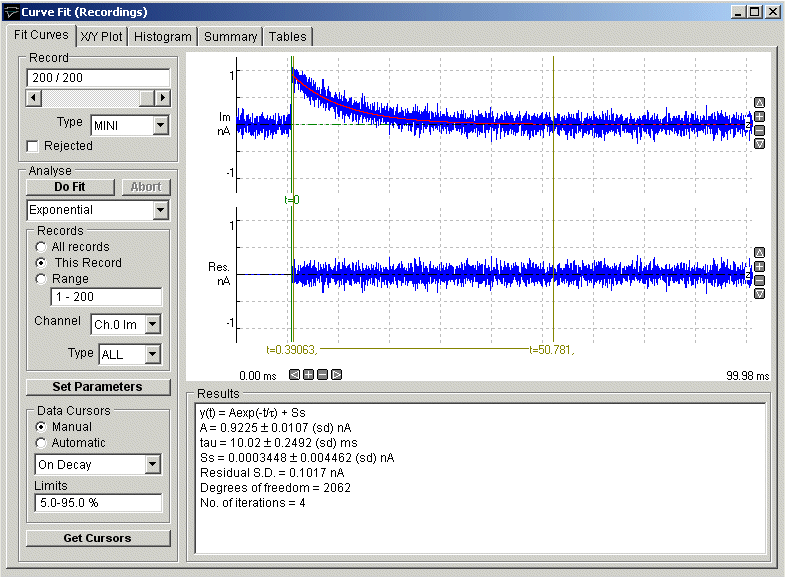
1) Select the Curve Fit page by clicking on its page tab.
2) Select the equation to be fitted to the record(s).
3) Select the channel containing the signal waveform to which the curve is to be fitted, from the Channel list.
4) Define the range of records to be analysed, by selecting All Records to analyse all records, or This Record to analyses only the currently displayed record, or Range and enter a range of records.
5) Select the type of records to be measured by selecting an option from the Type list. Select ALL to measure records of any type (except rejected records).
6) Select Manual or Automatic Data Cursors mode. In manual mode, the region within the signal to which the curve is to be fitted is set manually using a set of 3 cursors on the display. In automatic mode, the cursors are set automaticall automatically.
7) If you have selected Automatic Data Cursor mode, select On Rise, On Decay or Rise+Decay, to determine whether the cursors are to be placed on the rising phase, decaying phase, or complete time course of the signal waveform. Then enter the levels on the waveform where the cursors are to be placed in the Limits box. (Default setting is 10-90%, placing the cursors at 10% and 90% of peak amplitude on the selected phase)
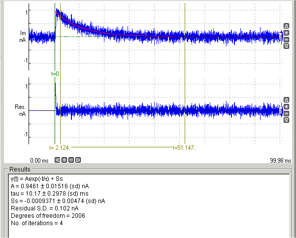
8) If you have selected Manual Data Cursors mode, define the curve fitting region by using three vertical cursors – two (blue, marked |) define the region to which the equation is to be fitted, the third (green, marked t0) defines where the zero time points for the equation is.
(Note that the choice of fitting region depends upon the kind of curve being fitted. Sometimes, only part of the signal is chosen, such as when an exponential curve is to be fitted to the decay phase of the signal. In the example shown here, the fitting region cursors have been placed on the decay phase of an endplate current. Zero time (t0) has been defined at the onset of the signal.)
9) If you wish to change the initial values for the equation parameters, or fix some parameters so they do not change during the fit, click the Set Parameters button to open the Set Fitting Parameters dialog box.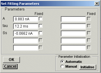
If you want to keep a parameter fixed at a set value, enter the value into the appropriate parameter box and click the Fixed check box.
10) When all curve fitting settings have been made, click the Do Fit button to initiate the curve fitting sequence.
The iterative curve fitting process now begins. The SSQMIN routine iterates through a variety of trial parameter sets, until no more improvement can be obtained. The number of iterations are displayed as fitting progresses. The best fit is usually found within 10-20 iterations. Fitting is aborted if the process has not converged to a suitable answer within 100 iterations, and can also be aborted by clicking the Abort button.
For each record fitted, the best fit curve is indicated by a red curve superimposed on the blue signal trace. A residuals trace is shown below indicating the difference between the fitted curve and the data. The parameters of the best fitting equation are shown in the Results table, along with the parameter standard error, the residual standard deviation (between the fitted and data points), statistical degrees of freedom in the fit, and the number of iterations it took to find the best fit.