|
Audience |
Beginner |
|
Length |
30 minutes |
|
Prerequisites |
None |
|
Script File |
|
Note
The most fundamental capability of GMAT is to propagate, or simulate the orbital motion of, spacecraft. The ability to propagate spacecraft is used in nearly every practical aspect of space mission analysis, from simple orbital predictions (e.g. When will the International Space Station be over my house?) to complex analyses that determine the thruster firing sequence required to send a spacecraft to the Moon or Mars.
This tutorial will teach you how to use GMAT to propagate a
spacecraft. You will learn how to configure
Spacecraft and Propagator
resources, and how to use the Propagate command to
propagate the spacecraft to orbit periapsis, which is the point of minimum
distance between the spacecraft and Earth. The basic steps in this
tutorial are:
-
Configure a
Spacecraftand define its epoch and orbital elements. -
Configure a
Propagator. -
Modify the default
OrbitViewplot to visualize the spacecraft trajectory. -
Modify the
Propagatecommand to propagate the spacecraft to periapsis. -
Run the mission and analyze the results.
In this section, you will rename the default
Spacecraft and set the
Spacecraft’s initial epoch and classical orbital
elements. You’ll need GMAT open, with the default mission loaded. To load
the default mission, click New Mission
( ) or start a new GMAT session.
-
In the Resources tree, right-click DefaultSC and click Rename.
-
Type
Sat. -
Click OK.
-
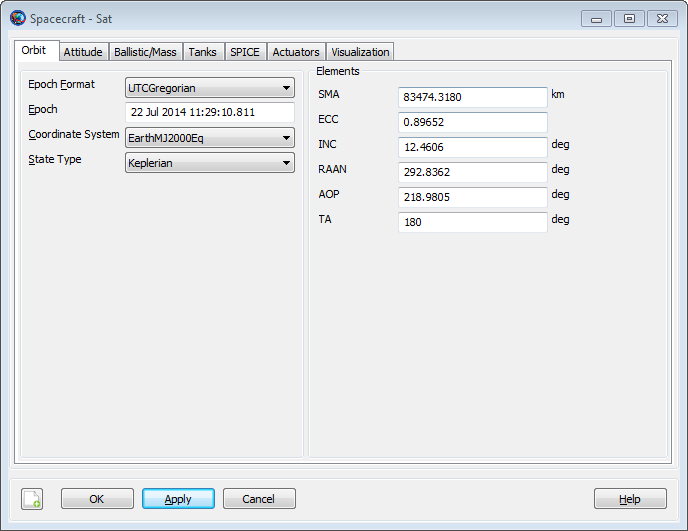
In the Resources tree, double-click Sat. Click the Orbit tab if it is not already selected.
-
In the Epoch Format list, select UTCGregorian. You’ll see the value in the Epoch field change to the UTC Gregorian epoch format.
-
In in the Epoch box, type
22
          Jul 2014 11:29:10.811
. This field is case-sensitive, and must be entered in the exact format shown. -
Click Apply or press the ENTER key to save these changes.
-
In the StateType list, select Keplerian. In the Elements list, you will see the GUI reconfigure to display the Keplerian state representation.
-
In the SMA box, type
83474.318. -
Set the remaining orbital elements as shown in the table below.
-
Click OK.
-
Click Save (
 ). If this is the first time you
have saved the mission, you’ll be prompted to provide a name and
location for the file.
). If this is the first time you
have saved the mission, you’ll be prompted to provide a name and
location for the file.
In this section you’ll rename the default
Propagator and configure the force model.
-
In the Resources tree, right-click DefaultProp and click Rename.
-
Type
LowEarthProp. -
Click OK.
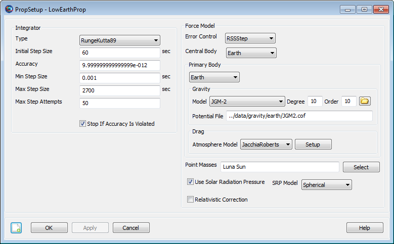
For this tutorial you will use an Earth 10×10 spherical harmonic model, the Jacchia-Roberts atmospheric model, solar radiation pressure, and point mass perturbations from the Sun and Moon.
-
In the Resources tree, double-click LowEarthProp.
-
Under Gravity, in the Degree box, type
10. -
In the Order box, type
10. -
In Atmosphere Model list, click JacchiaRoberts.
-
Click the Select button next to the Point Masses box. This opens the CelesBodySelectDialog window.
-
In the Available Bodies list, click Sun, then click -> to add Sun to the Selected Bodies list.
-
Add the moon (named Luna in GMAT) in the same way.
-
Click OK to close the CelesBodySelectDialog.
-
Select Use Solar Radiation Pressure to toggle it on. Your screen should now match Figure 5.2, “Force Model Configuration”.
-
Click OK.
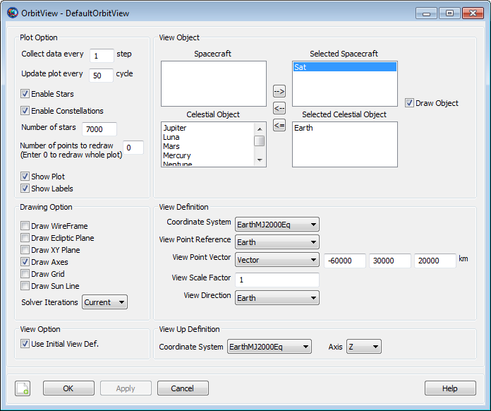
Now you will configure an OrbitView plot so
you can visualize Sat and its trajectory. The orbit
of Sat is highly eccentric. To view the entire
orbit at once, we need to adjust the settings of
DefaultOrbitView.
-
In the Resources tree, double-click DefaultOrbitView.
-
In the three boxes to the right of View Point Vector, type the values
-60000,30000, and20000respectively. -
Under Drawing Option to the left, clear Draw XY Plane. Your screen should now match Figure 5.3, “DefaultOrbitView Configuration”.
-
Click OK.
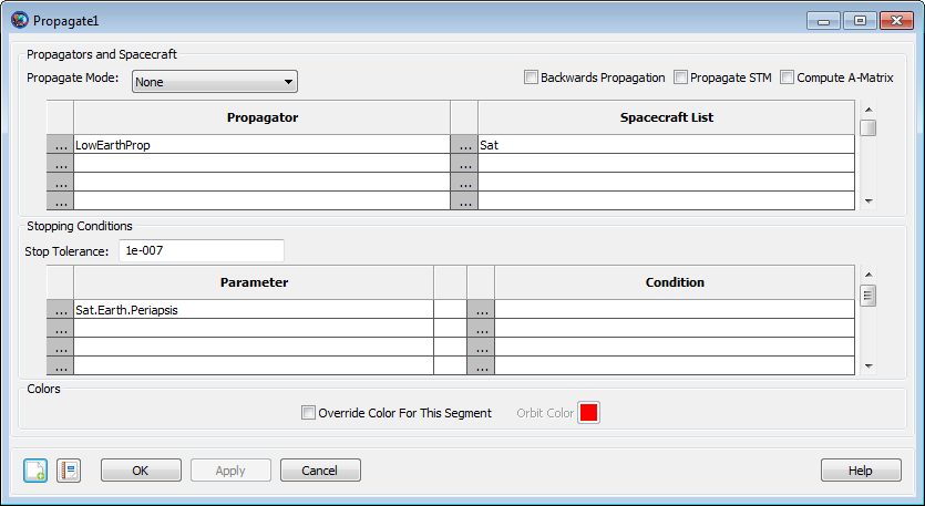
This is the last step before running the mission. Below you will configure a Propagate command to propagate (or simulate the motion of) Sat to orbit periapsis.
-
Click the Mission tab to display the Mission tree.
-
Double-click Propagate1.
-
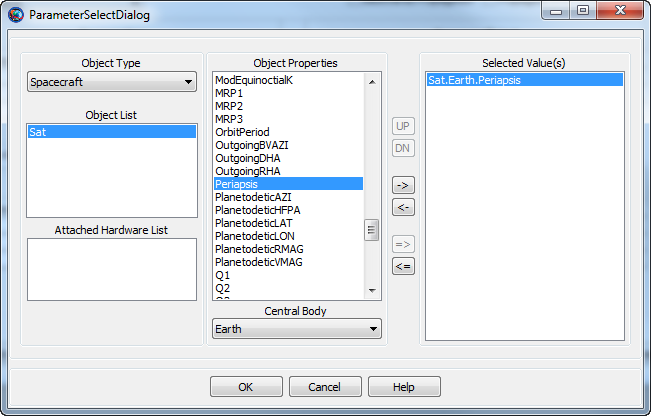
Under Stopping Conditions, click the (...) button to the left of Sat.ElapsedSecs. This will display the ParameterSelectDialog window.
-
In the Object List box, click Sat if it is not already selected. This directs GMAT to associate the stopping condition with the spacecraft Sat.
-
In the Object Properties list, double-click Periapsis to add it to the Selected Values list. This is shown in Figure 5.4, “Propagate Command ParameterSelectDialog Configuration”.
-
Click OK. Your screen should now match Figure 5.5, “Propagate Command Configuration”.
-
Click OK.
Congratulations, you have now configured your first GMAT mission and are ready to run the mission and analyze the results.
-
Click Save (
) to save your mission. -
Click the Run (
 ).
).
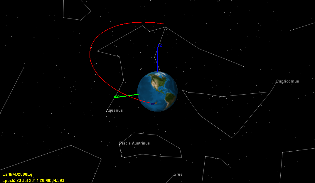
You will see GMAT propagate the orbit and stop at orbit periapsis. Figure 5.6, “Orbit View Plot after Mission Run” illustrates what you should see after correctly completing this tutorial. Here are a few things you can try to explore the results of this tutorial:
-
Manipulate the DefaultOrbitView plot using your mouse to orient the trajectory so that you can to verify that at the final location the spacecraft is at periapsis. See the OrbitView reference for details.
-
Display the command summary:
-
Click the Mission tab to display the Mission tree.
-
Right-click Propagate1 and select Command Summary to see data on the final state of Sat.
-
Use the Coordinate System list to change the coordinate system in which the data is displayed.
-
-
Click Start Animation (
 ) to animate the mission and watch
the orbit propagate from the initial state to periapsis.
) to animate the mission and watch
the orbit propagate from the initial state to periapsis.