|
Audience |
Advanced |
|
Length |
90 minutes |
|
Prerequisites |
Complete Simulating an Orbit, Simple Orbit Transfer, Mars B-Plane Targeting tutorial and take GMAT Fundamentals training course or watch videos |
|
Script File |
|
Note
For highly elliptic earth orbits (HEO), it is often cheaper to use the Moon’s gravity to raise periapsis or to perform plane changes, than it is to use the spacecraft’s propulsion resources. However, designing lunar flyby’s to achieve multiple specific mission constraints is non-trivial and requires modern optimization techniques to minimize fuel usage while simultaneously satisfying trajectory constraints. In this tutorial, you will learn how to design flyby trajectories by writing a GMAT script to perform multiple shooting optimization. As the analyst, your goal is to design a lunar flyby that provides a mission orbit periapsis of TBD km and changes the inclination of the mission orbit to TBD degrees. (Note: There are other mission constraints that will be discussed in more detail below.)
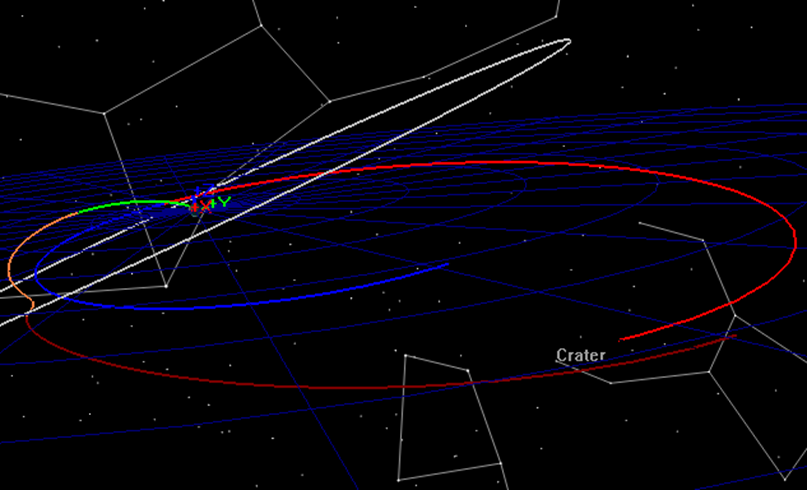
To efficiently solve the problem, we will employ the Multiple Shooting Method to break down the sensitive boundary value problem into smaller, less sensitive problems. We will employ three trajectory segments. The first segment will begin at Transfer Orbit Insertion (TOI) and will propagate forward; the second segment is centered at lunar periapsis and propagates both forward and backwards. The third segment is centered on Mission Orbit Insertion (MOI) and propagates forwards and backwards. See figures 1 and 2 that illustrate the final orbit solution and the “Control Points” and “Patch Points” used to solve the problem.
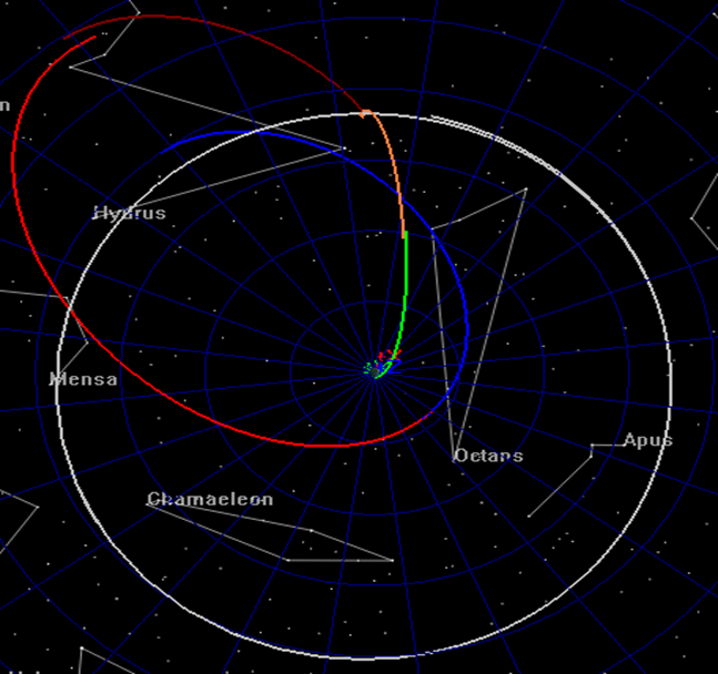
To begin this tutorial we start with a several views of the solution to provide a physical understanding of the problem. In Fig. 1, an illustration of a lunar flyby is shown with the trajectory displayed in red and the Moon’s orbit displayed in yellow. The Earth is at the center of the frame. We require that the following constraints are satisfied at TOI:
-
The spacecraft is at orbit perigee,
-
The spacecraft is at an altitude of 285 km.
-
The inclination of the transfer orbit is 28.5 degrees.
At lunar flyby, we only require that the flyby altitude is greater than 100 km. This constraint is satisfied implicitly so we will not explicitly script this constraint. An insertion maneuver is performed at earth perigee after the lunar fly to insert into the mission orbit. The following constraints must be satisfied after MOI.
-
The mission orbit perigee is 15 Earth radii.
-
The mission orbit apogee is 60 Earth radii.
-
The mission orbit inclination is 10 degrees.
Note: (Phasing with the moon is important for these orbits but design considerations for lunar phasing are beyond the scope of this tutorial)
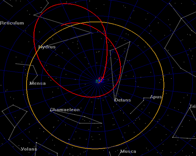
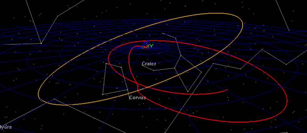
Figure 3 illustrates the mission timeline and how control points and patch points are defined. Control points are drawn using a solid blue circle and are defined as locations where the state of the spacecraft is treated as an optimization variable. Patch points are drawn with an empty blue circle and are defined as locations where position and/or velocity continuity is enforced. For this tutorial, we place control points at TOI, the lunar flyby and MOI. At each patch point, the six Cartesian state elements, and the epoch are varied for a total of 18 optimization variables. At the MOI patch point, there is an additional optimization variable for the delta V to
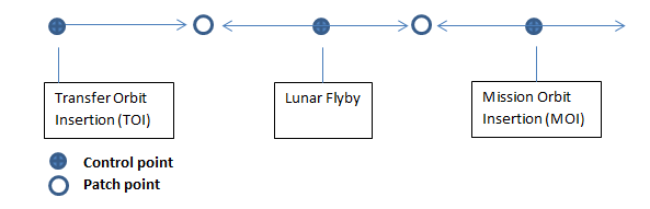
Notice that while there are only three patch points, we have 5 segments (which will result in 5 spacecraft). The state at the lunar flyby, which is defined as a control point, is propagated backwards to a patch point and forwards to a patch point. The same occurs for the MOI control point. To design this trajectory, you will need to create the following GMAT resources.
-
Create a Moon-centered coordinate system.
-
Create 5 spacecraft required for modeling segments.
-
Create an Earth-centered and a Moon-centered propagator.
-
Create an impulsive maneuver.
-
Create many user variables for use in the script.
-
Create A VF13ad optimizer.
-
Create plots for tracking the optimization process.
After creating the resources using script snippets you will construct the optimization sequence using GMAT script. Pseudo-code for the optimization sequence is shown below.
          Define optimization initial guesses
Initialize variables
Optimize
      Loop initializations
      Vary control point epochs
      Set epochs on spacecraft
      Vary control point state values
      Configure/initialize spacecraft
      Apply constraints on initial control points (i.e before propagation)
      Propagate spacecraft
      Apply patch point constraints
      Apply constraints on mission orbit
      Apply cost function
EndOptimize
After constructing the basic optimization sequence we will perform the following steps:
-
Run the sequence and analyze the initial guess.
-
Run the optimizer satisfying only the patch point constraints.
-
Turn on the mission orbit constraints and find a feasible solution.
-
Use the feasible solution as the initial guess and find an optimal solution.
-
Apply an altitude constraint at lunar orbit periapsis
For this tutorial, you’ll need GMAT open, with a blank script editor open. To open a blank script editor, click the New Script button in the toolbar.
You will need a Moon-centered CoordinateSystem for the lunar flyby control point so we begin by creating an inertial system centered at the moon. Use the MJ2000Eq axes for this system.
            %----------------------------------------------------
% Configure coordinate systems
%----------------------------------------------------

Create CoordinateSystem MoonMJ2000Eq
MoonMJ2000Eq.Origin = Luna
MoonMJ2000Eq.Axes   = MJ2000Eq
You will need 5 Spacecraft for this mission design. The epoch and state information will be set in the mission sequence and here we only need to configure coordinate systems for the Spacecraft. The Spacecraft named satTOI models the transfer orbit through the first patch point. Use the EarthMJ200Eq CoordinateSystem for satTOI. satFlyBy_Forward and satFlyBy_Backward model the trajectory from the flyby backwards to patch point 1 and forward to patch point 2 respectively. Use the MoonMJ2000Eq CoordinateSystem for satFlyBy_Forward and satFlyBy_Backward. Similarly, satMOI_Forward and satMOI_Backward model the trajectory on either side of the MOI maneuver. Use the MoonMJ2000Eq CoordinateSystem for satMOI_Forward and satMOI_Backward.
            %----------------------------------------------------
% Configure spacecraft
%----------------------------------------------------

%  The TOI control point
Create Spacecraft satTOI
satTOI.DateFormat                  = TAIModJulian
satTOI.CoordinateSystem            = EarthMJ2000Eq

%  Flyby control point
Create Spacecraft satFlyBy_Forward
satFlyBy_Forward.DateFormat        = TAIModJulian
satFlyBy_Forward.CoordinateSystem  = MoonMJ2000Eq

%  Flyby control point
Create Spacecraft satFlyBy_Backward
satFlyBy_Backward.DateFormat       = TAIModJulian
satFlyBy_Backward.CoordinateSystem = MoonMJ2000Eq

% MOI control point
Create Spacecraft satMOI_Backward
satMOI_Backward.DateFormat         = TAIModJulian
satMOI_Backward.CoordinateSystem   = EarthMJ2000Eq

% MOI control point
Create Spacecraft satMOI_Forward
satMOI_Forward.DateFormat          = TAIModJulian
satMOI_Forward.CoordinateSystem    = EarthMJ2000Eq
Modeling the motion of the spacecraft when near the earth and near the moon requires two propagators; one Earth-centered, and one Moon-centered. The script below configures the ForceModel named NearEarthForceModel to use JGM-2 8x8 harmonic gravity model, with point mass perturbations from the Sun and Moon, and the SRP perturbation. The ForceModel named NearMoonForceModel is similar but uses point mass gravity for all bodies. Note that the integrators are configured for performance and not for accuracy to improve run times for the tutorial. There are times when integrator accuracy can cause issues with optimizer performance due to noise in the numerical solutions.
            %----------------------------------------------------
% Configure propagators and force models
%----------------------------------------------------

Create ForceModel NearEarthForceModel
NearEarthForceModel.CentralBody               = Earth
NearEarthForceModel.PrimaryBodies             = {Earth}
NearEarthForceModel.PointMasses               = {Luna, Sun}
NearEarthForceModel.SRP                       = On
NearEarthForceModel.GravityField.Earth.Degree = 8
NearEarthForceModel.GravityField.Earth.Order  = 8

Create ForceModel NearMoonForceModel
NearMoonForceModel.CentralBody                = Luna
NearMoonForceModel.PointMasses                = {Luna, Earth, Sun}
NearMoonForceModel.Drag                       = None
NearMoonForceModel.SRP                        = On
            Create Propagator NearEarthProp
NearEarthProp.FM = NearEarthForceModel
NearEarthProp.Type                     = PrinceDormand78
NearEarthProp.InitialStepSize          = 60
NearEarthProp.Accuracy                 = 1e-11
NearEarthProp.MinStep                  = 0.0
NearEarthProp.MaxStep                  = 86400

Create Propagator NearMoonProp
NearMoonProp.FM                        = NearMoonForceModel
NearMoonProp.Type                      = PrinceDormand78
NearMoonProp.InitialStepSize           = 60
NearMoonProp.Accuracy                  = 1e-11
NearMoonProp.MinStep                   = 0
NearMoonProp.MaxStep                   = 86400
We will require one ImpulsiveBurn to insert the spacecraft into the mission orbit. Define the maneuver as MOI and configure the maneuver to be applied in the VNB (Earth-referenced) Axes.
            %----------------------------------------------------
% Configure maneuvers
%----------------------------------------------------

Create ImpulsiveBurn MOI
MOI.CoordinateSystem   = Local
MOI.Origin             = Earth
MOI.Axes               = VNB
IThe optimization sequence requires many user variables that will be discussed in detail later in the tutorial when we define those variables. For now, we simply create the variables (which initializes them to zero). The naming convention used here is that variables used to define constraint values begin with “con”. For example, the variable used to define the constraint on TOI inclination is called conTOIInclination. Variables beginning with “error” are used to compute constraint variances. For example, the variable used to define the error in MOI inclination is called errorTOIInclination.
            %----------------------------------------------------
% Create user data: variables, arrays, strings
%----------------------------------------------------

%  Variables for defining constraint values
Create Variable conTOIPeriapsis conMOIPeriapsis conTOIInclination
Create Variable conLunarPeriapsis conMOIApoapsis conMOIInclination
Create Variable launchRdotV finalPeriapsisValue

%  Variables for computing constraint violations
Create Variable errorPos1 errorVel1 errorPos2 errorVel2
Create Variable errorMOIRadApo errorMOIRadPer errorMOIInclination

%  Variables for managing time calculations
Create Variable patchTwoElapsedDays patchOneEpoch patchTwoEpoch refEpoch
Create Variable toiEpoch flybyEpoch moiEpoch patchOneElapsedDays
Create Variable deltaTimeFlyBy

%  Constants and miscellaneous variables
Create Variable earthRadius earthMu launchEnergy launchVehicleDeltaV
Create Variable toiDeltaV launchCircularVelocity loopIdx Cost
The script below creates a VF13ad optimizer provided in the Harwell Subroutine Library. VF13ad is an Sequential Quadratic Programming (SQP) optimizer that uses a line search method to solve the Non-linear Programming Problem (NLP). Here we configure the optimizer to use forward differencing to compute the derivatives, define the maximum iterations to 200, and define convergence tolerances.
            %----------------------------------------------------
% Configure solvers
%----------------------------------------------------

Create VF13ad NLPOpt
NLPOpt.ShowProgress          = true
NLPOpt.ReportStyle           = Normal
NLPOpt.ReportFile            = 'VF13adVF13ad1.data'
NLPOpt.MaximumIterations     = 200
NLPOpt.Tolerance             = 1e-004
NLPOpt.UseCentralDifferences = false
NLPOpt.FeasibilityTolerance  = 0.1
You will need an OrbitView 3-D graphics window to visualize the trajectory and especially the initial guess. Below we configure an orbit view to view the entire trajectory in the EarthMJ2000Eq coordinate system. Note that we must add all five Spacecraft to the OrbitView. Updating an OrbitView during optimization can dramatically slow down the optimization process and they are best use to check initial configuration and then us XY plots to track numerical progress. Later in the tutorial, we will toggle the ShowPlot field to false once we have verified the initial configuration is correct.
            %----------------------------------------------------
% Configure plots, reports, etc.
%----------------------------------------------------

Create OrbitView EarthView
EarthView.ShowPlot               = true
EarthView.SolverIterations       = All
EarthView.UpperLeft              = ...
    [ 0.4960127591706539 0.00992063492063492 ];
EarthView.Size                   = ...
    [ 0.4800637958532695 0.5218253968253969 ];
EarthView.RelativeZOrder         = 501
EarthView.Add                    = ...
{satTOI, satFlyBy_Forward, satFlyBy_Backward, satMOI_Backward, ...
 Earth, Luna, satMOI_Forward}
EarthView.CoordinateSystem       = EarthMJ2000Eq
EarthView.DrawObject             = [ true true true true true]
EarthView.OrbitColor             = ...
[ 255 32768 1743054 16776960 32768 12632256 14268074 ]
EarthView.TargetColor            = ...
[ 65280 124 4227327 255 12345 9843 16711680 ];
EarthView.DataCollectFrequency   = 1
EarthView.UpdatePlotFrequency    = 50
EarthView.NumPointsToRedraw      = 300
EarthView.ViewScaleFactor        = 35
EarthView.ViewUpAxis             = X
EarthView.UseInitialView         = On
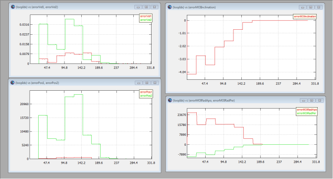
Below we create several XYPlots and a ReportFile. We will use XYPlots to monitor the progress of the optimizer in satisfying constraints. PositionError1 plots the position error at the first patch point... VelocityError2 plots the velocity error at the second patch point, and so on. OrbitDimErrors plots the errors in the periapsis and apoapsis radii for the mission orbit. When optimization is proceeding as expected, these plots should show errors driven to zero.
            Create XYPlot PositionError
PositionError.SolverIterations = All
PositionError.UpperLeft        = [ 0.02318840579710145 0.4358208955223881 ];
PositionError.Size             = [ 0.4594202898550724 0.5283582089552239 ];
PositionError.RelativeZOrder   = 378
PositionError.XVariable        = loopIdx
PositionError.YVariables       = {errorPos1, errorPos2}
PositionError.ShowGrid         = true
PositionError.ShowPlot         = true

Create XYPlot VelocityError
VelocityError.SolverIterations = All
VelocityError.UpperLeft        = [ 0.02463768115942029 0.01194029850746269 ];
VelocityError.Size             = [ 0.4565217391304348 0.4208955223880597 ];
VelocityError.RelativeZOrder   = 410
VelocityError.XVariable        = loopIdx
VelocityError.YVariables       = {errorVel1, errorVel2}
VelocityError.ShowGrid         = true
VelocityError.ShowPlot         = true

Create XYPlot OrbitDimErrors
OrbitDimErrors.SolverIterations = All
OrbitDimErrors.UpperLeft      = [ 0.4960127591706539 0.5337301587301587 ];
OrbitDimErrors.Size           = [ 0.481658692185008 0.4246031746031746 ];
OrbitDimErrors.RelativeZOrder = 347
OrbitDimErrors.XVariable      = loopIdx
OrbitDimErrors.YVariables     = {errorMOIRadApo, errorMOIRadPer}
OrbitDimErrors.ShowGrid       = true
OrbitDimErrors.ShowPlot       = true

Create XYPlot IncError
IncError.SolverIterations = All
IncError.UpperLeft        = [ 0.4953586497890296 0.01306240928882438 ];
IncError.Size             = [ 0.479324894514768 0.5079825834542816 ];
IncError.RelativeZOrder   = 382
IncError.YVariables       = {errorMOIInclination}
IncError.XVariable        = loopIdx
IncError.ShowGrid         = true
IncError.ShowPlot         = true
Create a ReportFile to allow reporting useful information to a text file for review after the optimization process is complete.
            Create ReportFile debugData
debugData.SolverIterations = Current
debugData.Precision        = 16
debugData.WriteHeaders     = Off
debugData.LeftJustify      = On
debugData.ZeroFill         = Off
debugData.ColumnWidth      = 20
debugData.WriteReport      = false
Now that the resources are created and configured, we will construct the optimization sequence. Pseudo-script for the optimization sequence is shown below. We will start by defining initial guesses for the control point optimization variables. Next, selected variables are initialized. Take some time and study the structure of the optimization loop before moving on to the next step.
            Define optimization initial guesses
Initialize variables
Optimize
      Loop initializations
      Vary control point epochs
      Set epochs on spacecraft
      Vary control point state values
      Set state values on spacecraft
      Apply constraints on control points (i.e before propagation)
      Propagate spacecraft
      Apply patch point constraints (i.e. after propagation)
      Apply constraints on mission orbit
      Apply cost function
EndOptimize
Below we define initial guesses for the optimization variables. Initial guesses are often difficult to generate and to ensure you can take this tutorial we have provided a reasonable initial guess for this problem. You can use GMAT to produce initial guesses and the sample script named Ex_GivenEpochGoToTheMoon distributed with GMAT can be used for that purpose for this tutorial.
The time variables launchEpoch, flybyEpoch and moiEpoch are the TAI modified Julian epochs of the launch, flyby, and MOI. It is not obvious yet that these are TAI modified Julian epochs, but later we use statements like this to set the epoch: satTOI.Epoch.TAIModJulian = launchEpoch. Recall that we previously set up the spacecraft to used coordinate systems appropriate to the problem. Setting satTOI.X sets the quantity in EarthMJ2000Eq and satFlyBy_Forward.X sets the quantity in MoonMJ2000Eq because of the configuration of the spacecraft.
            BeginMissionSequence

%  Define initial guesses for optimization variables
BeginScript 'Initial Guess Values'

   %  Robust intial guess but not feasible
   toiEpoch = 27698.1612435
   flybyEpoch = 27703.7658714
   moiEpoch = 27723.305398
   satTOI.X = -6659.70273964
   satTOI.Y = -229.327053112
   satTOI.Z = -168.396030559
   satTOI.VX = 0.26826479315
   satTOI.VY = -9.54041067213
   satTOI.VZ = 5.17141415746
   satFlyBy_Forward.X = 869.478955662
   satFlyBy_Forward.Y = -6287.76679557
   satFlyBy_Forward.Z = -3598.47087228
   satFlyBy_Forward.VX = 1.14619150302
   satFlyBy_Forward.VY = -0.73648611256
   satFlyBy_Forward.VZ = -0.624051812914
   satMOI_Backward.X = -53544.9703742
   satMOI_Backward.Y = -68231.6310266
   satMOI_Backward.Z = -1272.76362793
   satMOI_Backward.VX = 2.051823425
   satMOI_Backward.VY = -1.91406286218
   satMOI_Backward.VZ = -0.280408526046
   MOI.Element1 = -0.0687322937282

EndScript
The script below is used to define some constants and to define the values for various constraints applied to the trajectory. Pay particular attention to the constraint values and time values. For example, the variable conTOIPeriapsis defines the periapsis radius at launch constraint to be at about 285 km (geodetics will cause altitude to vary slightly). The variable conMOIApoapsis defines the mission orbit apoapsis to be 60 earth radii. The variables patchOneElapsedDays, patchTwoElapsedDays, and refEpoch are particularly important as they define the epochs of the patch points later in the script using lines like this patchOneEpoch = refEpoch + patchOneElapsedDayspatchOneEpoch. The preceding line defines the epoch of the first patch point to be one day after refEpoch (refEpoch is set to launchEpoch). Similarly, the epoch of the second patch point is defined as 13 days after refEpoch. Note, the patch point epochs can be treated as optimization variables but that was not done to reduce complexity of the tutorial.
            %  Define constants and configuration settings
BeginScript 'Constants and Init'

   %  Some constants
   earthRadius          = 6378.1363

   %  Define constraint values and other constants
   conTOIPeriapsis     = 6378 + 285   % constraint on launch periapsis
   conTOIInclination   = 28.5         % constraint launch inclination
   conLunarPeriapsis   = 8000         % constraint on flyby altitude
   conMOIApoapsis      = 60*earthRadius  % constraint on mission apoapsis
   conMOIInclination   = 10              % constraint on mission inc.
   conMOIPeriapsis     = 15*earthRadius  % constraint on mission periapsis
   patchOneElapsedDays = 1               % define epoch of patch 1
   patchTwoElapsedDays = 13              % define epoch of patch 2
   refEpoch            = toiEpoch     % ref. epoch for time quantities

EndScript

%  The optimization loop
Optimize 'Optimize Flyby' NLPOpt ...
   {SolveMode = Solve, ExitMode = DiscardAndContinue}

   %   Loop initializations
   loopIdx = loopIdx + 1

EndOptimize
Caution
In the above script snippet, we have included the EndOptimize command so that your script will continue to build while we construct the optimization sequence. You must paste subsequence script snippets inside of the optimization loop.
Now we will write the commands that vary the control point epochs and apply those epochs to the spacecraft. The first three script lines below define launchEpoch, flybyEpoch, and moiEpoch to be optimization variables. It is important to note that when a Vary command is written like this
Vary NLPOpt(launchEpoch = launchEpoch, . . .
that you are telling the optimizer to vary launchEpoch (the RHS of the equal sign), and to use as the initial guess the value contained in launchEpoch when the command is first executed. This will allow us to easily change initial guess values and perform “Apply Corrections” via the script interface which will be shown later. Continuing with the script explanation, the last five lines below set the epochs of the spacecraft according to the optimization variables and set up the patch point epochs.
               %  Vary the epochs
   Vary NLPOpt(toiEpoch = toiEpoch, {Perturbation = 0.0001, MaxStep = 0.5})
   Vary NLPOpt(flybyEpoch = flybyEpoch,{Perturbation=0.0001,MaxStep=0.5})
   Vary NLPOpt(moiEpoch = moiEpoch, {Perturbation = 0.0001,MaxStep=0.5})

   %  Configure epochs and spacecraft
   satTOI.Epoch.TAIModJulian           = toiEpoch
   satMOI_Backward.Epoch.TAIModJulian  = moiEpoch
   satFlyBy_Forward.Epoch.TAIModJulian = flybyEpoch
   patchOneEpoch                       = refEpoch + patchOneElapsedDays
   patchTwoEpoch                       = refEpoch + patchTwoElapsedDays
The script below defines the control point optimization variables and defines the initial guess values for each optimization variable. For example, the following line
Vary NLPOpt(satTOI.X = satTOI.X, {Perturbation =
      0.00001, MaxStep = 100})
tells GMAT to vary the X Cartesian value of satTOI using as the initial guess the value of satTOI.X at initial command execution. The Perturbation used to compute derivatives is 0.00001 and the optimizer will not take steps larger than 100 for this variable. Note: units of settings like Perturbation are the same as the unit for the optimization variable.
Notice the lines at the bottom of this script snippet that look like this:
satFlyBy_Backward = satFlyBy_Forward
This line assigns an entire Spacecraft to another Spacecraft. Because we are varying one control point in the middle of a segment, this assignment allows us to conveniently set the second Spacecraft without independently varying its state properties.
               %  Vary the states and delta V
   Vary NLPOpt(satTOI.X            = ...
   satTOI.X, {Perturbation = 0.00001, MaxStep = 100})
   Vary NLPOpt(satTOI.Y            = ...
   satTOI.Y, {Perturbation = 0.000001, MaxStep = 100})
   Vary NLPOpt(satTOI.Z            = ...
   satTOI.Z, {Perturbation = 0.00001, MaxStep = 100})
   Vary NLPOpt(satTOI.VX           = ...
   satTOI.VX, {Perturbation = 0.00001, MaxStep = 0.05})
   Vary NLPOpt(satTOI.VY           = ...
   satTOI.VY, {Perturbation = 0.000001, MaxStep = 0.05})
   Vary NLPOpt(satTOI.VZ           = ...
   satTOI.VZ, {Perturbation = 0.000001, MaxStep = 0.05})
   Vary NLPOpt(satFlyBy_Forward.X  = ...
   satFlyBy_Forward.MoonMJ2000Eq.X, {Perturbation = 0.00001, MaxStep = 100})
   Vary NLPOpt(satFlyBy_Forward.Y  = ...
   satFlyBy_Forward.MoonMJ2000Eq.Y, {Perturbation = 0.00001, MaxStep = 100})
   Vary NLPOpt(satFlyBy_Forward.Z  = ...
   satFlyBy_Forward.MoonMJ2000Eq.Z, {Perturbation = 0.00001, MaxStep = 100})
   Vary NLPOpt(satFlyBy_Forward.VX = ...
   satFlyBy_Forward.MoonMJ2000Eq.VX, {Perturbation = 0.00001, MaxStep = 0.1})
   Vary NLPOpt(satFlyBy_Forward.VY = ...
   satFlyBy_Forward.MoonMJ2000Eq.VY, {Perturbation = 0.00001, MaxStep = 0.1})
   Vary NLPOpt(satFlyBy_Forward.VZ = ...
   satFlyBy_Forward.MoonMJ2000Eq.VZ, {Perturbation = 0.00001, MaxStep = 0.1})
   Vary NLPOpt(satMOI_Backward.X   = ...
   satMOI_Backward.X, {Perturbation = 0.000001, MaxStep = 40000})
   Vary NLPOpt(satMOI_Backward.Y   = ...
   satMOI_Backward.Y, {Perturbation = 0.000001, MaxStep = 40000})
   Vary NLPOpt(satMOI_Backward.Z   = ...
   satMOI_Backward.Z, {Perturbation = 0.000001, MaxStep = 40000})
   Vary NLPOpt(satMOI_Backward.VX  = ...
   satMOI_Backward.VX, {Perturbation = 0.00001, MaxStep = 0.1})
   Vary NLPOpt(satMOI_Backward.VY  = ...
   satMOI_Backward.VY, {Perturbation = 0.00001, MaxStep = 0.1})
   Vary NLPOpt(satMOI_Backward.VZ  = ...
   satMOI_Backward.VZ, {Perturbation = 0.00001, MaxStep = 0.1})
   Vary NLPOpt(MOI.Element1        = ...
   MOI.Element1, {Perturbation = 0.0001, MaxStep = 0.005})

   %  Initialize spacecraft and do some reporting
   satFlyBy_Backward = satFlyBy_Forward
   satMOI_Forward    = satMOI_Backward
   deltaTimeFlyBy    = flybyEpoch - toiEpoch
Now that the control points have been set, we can apply constraints that occur at the control points (i.e. before propagation to the patch point). Notice below that the NonlinearContraint commands are commented out. We will uncomment those constraints later. The commands below, when uncommented, will apply constraints on the launch inclination, the launch periapsis radius, the mission orbit periapsis, and the last constraint ensures that TOI occurs at periapsis of the transfer orbit.
                %  Apply constraints on initial states
   %NonlinearConstraint NLPOpt(satTOI.INC=conTOIInclination)
   %NonlinearConstraint NLPOpt(satTOI.RadPer=conTOIPeriapsis)
   %NonlinearConstraint NLPOpt(satMOI_Backward.RadPer = conMOIPeriapsis)
   errorMOIRadPer = satMOI_Backward.RadPer - conMOIPeriapsis

   %  This constraint ensures that satTOI state is at periapsis at injection
   launchRdotV = (satTOI.X *satTOI.VX + satTOI.Y *satTOI.VY + ...
   satTOI.Z *satTOI.VZ)/1000
   %NonlinearConstraint NLPOpt(launchRdotV=0)
We are now ready to propagate the spacecraft to the patch points. We must propagate satTOI forward to patchOneEpoch, propagate satFlyBy_Backward backwards to patchOneEpoch, propagate satFlyBy_Forward to patchTwoEpoch, and propagate satMOI_Backward to patchTwoEpoch. Notice that some Propagate commands are applied inside of If statements to ensure that propagation is performed in the correct direction.%
            %  DO NOT PASTE THESE LINES INTO THE SCRIPT, THEY ARE
%  INCLUDED IN THE COMPLETE SNIPPET LATER IN THIS SECTION
If satFlyBy_Forward.TAIModJulian > patchTwoEpoch
      Propagate BackProp NearMoonProp(satFlyBy_Forward) . . .
   Else
      Propagate NearMoonProp(satFlyBy_Forward) . . .
EndIf
If In the script below, you will notice like this:
            %  DO NOT PASTE THESE LINES INTO THE SCRIPT, THEY ARE
%  INCLUDED IN THE COMPLETE SNIPPET LATER IN THIS SECTION
Propagate NearEarthProp(satTOI) {satTOI.TAIModJulian = patchOneEpoch, …
PenUp EarthView    %  The next three lines handle plot epoch discontinuity
Propagate BackProp NearMoonProp(satFlyBy_Backward)
PenDown EarthView
These lines are used to clean up discontinuities in the OrbitView that occur because we are making discontinuous changes to time in this complex script.
            %  Propagate the segments
   Propagate NearEarthProp(satTOI) {satTOI.TAIModJulian = ...
    patchOneEpoch, StopTolerance = 1e-005}
   PenUp EarthView  %  The next three lines handle discontinuity in plots
   Propagate BackProp NearMoonProp(satFlyBy_Backward)
   PenDown EarthView
   Propagate BackProp NearMoonProp(satFlyBy_Backward)...
   {satFlyBy_Backward.TAIModJulian = patchOneEpoch, StopTolerance = 1e-005}

   %  Propagate FlybySat to Apogee and apply apogee constraints
   PenUp EarthView  %  The next three lines handle discontinuity in plots
   Propagate NearMoonProp(satFlyBy_Forward)
   PenDown EarthView
   Propagate NearMoonProp(satFlyBy_Forward) ...
   {satFlyBy_Forward.Earth.Apoapsis, StopTolerance = 1e-005}
   Report debugData satFlyBy_Forward.RMAG

   %  Propagate FlybSat and satMOI_Backward to patchTwoEpoch
   If satFlyBy_Forward.TAIModJulian > patchTwoEpoch
      Propagate BackProp NearMoonProp(satFlyBy_Forward)...
   {satFlyBy_Forward.TAIModJulian = patchTwoEpoch, StopTolerance = 1e-005}
   Else
      Propagate NearMoonProp(satFlyBy_Forward)...
   {satFlyBy_Forward.TAIModJulian = patchTwoEpoch, StopTolerance = 1e-005}
   EndIf
   PenUp EarthView    %  The next three lines handle discontinuity in plots
   Propagate BackProp NearMoonProp(satMOI_Backward)
   PenDown EarthView
   Propagate BackProp NearMoonProp(satMOI_Backward)...
  {satMOI_Backward.TAIModJulian = patchTwoEpoch, StopTolerance = 1e-005}
The variables errorPos1 and others below are used in XYPlots to display position and velocity errors at the patch points.
               %  Compute constraint errors for plots
   errorPos1 = sqrt((satTOI.X - satFlyBy_Backward.X)^2 + ...
   (satTOI.Y - satFlyBy_Backward.Y)^2 + (satTOI.Z - satFlyBy_Backward.Z)^2)
   errorVel1 = sqrt((satTOI.VX - satFlyBy_Backward.VX)^2 + ...
   (satTOI.VY-satFlyBy_Backward.VY)^2+(satTOI.VZ-satFlyBy_Backward.VZ)^2)
   errorPos2 = sqrt((satMOI_Backward.X - satFlyBy_Forward.X)^2 + ...
   (satMOI_Backward.Y - satFlyBy_Forward.Y)^2 + ...
   (satMOI_Backward.Z - satFlyBy_Forward.Z)^2)
   errorVel2 = sqrt((satMOI_Backward.VX - satFlyBy_Forward.VX)^2 + ...
   (satMOI_Backward.VY - satFlyBy_Forward.VY)^2 + ...
   (satMOI_Backward.VZ - satFlyBy_Forward.VZ)^2)
The NonlinearConstraint commands below apply the patch point constraints.
               %  Apply the collocation constraints constraints on final states
   NonlinearConstraint NLPOpt(satTOI.EarthMJ2000Eq.X=...
   satFlyBy_Backward.EarthMJ2000Eq.X)
   NonlinearConstraint NLPOpt(satTOI.EarthMJ2000Eq.Y=...
   satFlyBy_Backward.EarthMJ2000Eq.Y)
   NonlinearConstraint NLPOpt(satTOI.EarthMJ2000Eq.Z=...
   satFlyBy_Backward.EarthMJ2000Eq.Z)
   NonlinearConstraint NLPOpt(satTOI.EarthMJ2000Eq.VX=...
   satFlyBy_Backward.EarthMJ2000Eq.VX)
   NonlinearConstraint NLPOpt(satTOI.EarthMJ2000Eq.VY=...
   satFlyBy_Backward.EarthMJ2000Eq.VY)
   NonlinearConstraint NLPOpt(satTOI.EarthMJ2000Eq.VZ=...
   satFlyBy_Backward.EarthMJ2000Eq.VZ)
   NonlinearConstraint NLPOpt(satMOI_Backward.EarthMJ2000Eq.X=...
   satFlyBy_Forward.EarthMJ2000Eq.X)
   NonlinearConstraint NLPOpt(satMOI_Backward.EarthMJ2000Eq.Y=...
   satFlyBy_Forward.EarthMJ2000Eq.Y)
   NonlinearConstraint NLPOpt(satMOI_Backward.EarthMJ2000Eq.Z=...
   satFlyBy_Forward.EarthMJ2000Eq.Z)
   NonlinearConstraint NLPOpt(satMOI_Backward.EarthMJ2000Eq.VX=...
   satFlyBy_Forward.EarthMJ2000Eq.VX)
   NonlinearConstraint NLPOpt(satMOI_Backward.EarthMJ2000Eq.VY=...
   satFlyBy_Forward.EarthMJ2000Eq.VY)
   NonlinearConstraint NLPOpt(satMOI_Backward.EarthMJ2000Eq.VZ=...
   satFlyBy_Forward.EarthMJ2000Eq.VZ)
We can now apply constraints on the final mission orbit that cannot be applied until after propagation. The script snippet below applies the inclination constraint on the final mission orbit, and applies the apogee radius constraint on the final mission orbit after MOI is applied.
               %  Apply mission orbit constraints/others on segments after propagation
   errorMOIInclination = satMOI_Forward.INC - conMOIInclination
   %NonlinearConstraint NLPOpt(satMOI_Forward.EarthMJ2000Eq.INC = ...
   % conMOIInclination)
      %  Propagate satMOI_Forward to apogee
   PenUp EarthView    %  The next three lines handle discontinuity in plots
   Propagate NearEarthProp(satMOI_Forward)
   PenDown EarthView
   If satMOI_Forward.Earth.TA > 180
     Propagate NearEarthProp(satMOI_Forward){satMOI_Forward.Earth.Periapsis}
   Else
      Propagate BackProp NearEarthProp(satMOI_Forward)...
      {satMOI_Forward.Earth.Periapsis}
   EndIf
   Maneuver MOI(satMOI_Forward)
   Propagate NearEarthProp(satMOI_Forward) {satMOI_Forward.Earth.Apoapsis}
   %NonlinearConstraint NLPOpt(satMOI_Forward.RadApo=conMOIApoapsis)
   errorMOIRadApo = satMOI_Forward.Earth.RadApo - conMOIApoapsis
The last script snippet applies the cost function and a Stop command. The Stop command is so that we can QA your script configuration and make sure the initial guess is providing reasonable results before attempting optimization.
               %  Apply cost function and
   Cost = sqrt( MOI.Element1^2 + MOI.Element2^2 + MOI.Element3^2)
   %Minimize NLPOpt(Cost)

   %  Report stuff at the end of the loop
   Report debugData MOI.Element1
   Report debugData satMOI_Forward.RMAG conMOIApoapsis conMOIInclination

   Stop
We are now ready to design the trajectory. We’ll do this in a couple of steps:
-
Run the script configuration and verify your configuration.
-
Run the mission applying only the patch point constraints to provide a smooth trajectory.
-
Run the mission with all constraints applied generating an optimal solution.
-
Run the mission with an alternative initial guess.
-
Add a new constraint and rerun the mission.
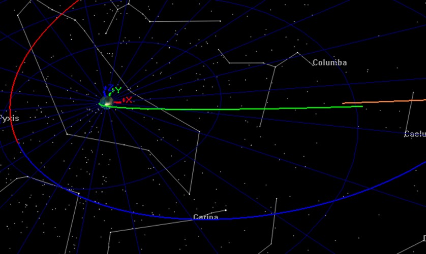
If your script is configured correctly, when you click Save-Sync-Run in the bottom of the script editor, you should see an OrbitView graphics window display the initial guess for the trajectory as shown below. In the graphics, satTOI is displayed in green, satFlyBy_Backward is displayed in orange, satFlyBy_Forward is displayed in dark red, and satMOI_Backward is displayed in bright red, and satMOI_Forward is displayed in blue.
You can use the mouse to manipulate the OrbitView to see that the patch points are indeed discontinuous for the initial guess as shown below in the two screen captures. If your configuration does not provide you with similar graphics, compare your script to the one provided for this tutorial and address any differences.
At this point in the tutorial, your script is configured to eliminate the patch point discontinuities but does not apply mission constraints. We need to make a few small modifications before proceeding. We will turn off the OrbitView to improve the run time, and we will remove the Stop command so that the optimizer will attempt to find a solution.
-
Near the bottom of the script, comment out the Stop command.
-
In the configuration of EarthView, change ShowPlot to false.
-
Click Save Sync Run.
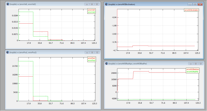
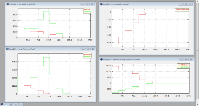
After a few optimizer iterations you should see “NLPOpt converged to within target accuracy" displayed in the GMAT message window and your XY plot graphics should appear as shown below. Let’s discuss the content of these windows. The upper left window shows the RSS history of velocity error at the two patch points during the optimization process. The lower left window shows the RSS history of the position error. The upper right window shows error in mission orbit inclination, and the lower right window shows error mission orbit apogee and perigee radii. You can see that in all cases the patch point discontinuities were driven to zero, but since other constraints were not applied there are still errors in some mission constraints.
Before proceeding to the next step, go to the message window and copy and paste the final values of the optimization variables to a text editor for later use:
At this point in the tutorial, your script is configured to eliminate the patch point discontinuities but does not apply constraints. We need to make a few small modifications to the script to find an solution that meets the constraints.
-
Remove the “%” sign from the all NonlinearConstraint commands and the Minimize command:
NonlinearConstraint NLPOpt(satTOI.INC=conTOIInclination) NonlinearConstraint NLPOpt(satTOI.RadPer=conTOIPeriapsis) NonlinearConstraint NLPOpt(satMOI_Backward.RadPer = conMOIPeriapsis) NonlinearConstraint NLPOpt(launchRdotV=0) NonlinearConstraint NLPOpt(satMOI_Forward.EarthMJ2000Eq.INC =. . . NonlinearConstraint NLPOpt(satMOI_Forward.RadApo=conMOIApoapsis) Minimize NLPOpt(Cost) -
Click Save Sync Run.
The screen capture below shows the plots after optimization has been completed. Notice that the constraint errors have been driven to zero in the plots
Another way to verify that the constraints have been satisfied is to look in the message window where the final constraint variances are displayed as shown below. We could further reduce the variances by lowering the tolerance setting on the optimizer.
              Equality Constraint Variances:
      Delta satTOI.INC = 1.44773082411e-011
      Delta satTOI.RadPer = 7.08496372681e-010
      Delta satMOI_Backward.RadPer = -3.79732227884e-007
      Delta launchRdotV = -1.87725390788e-014
      Delta satTOI.EarthMJ2000Eq.X = 0.00037122167123
      Delta satTOI.EarthMJ2000Eq.Y = 2.79954474536e-005
      Delta satTOI.EarthMJ2000Eq.Z = 2.78138068097e-005
      Delta satTOI.EarthMJ2000Eq.VX = -3.87579257577e-009
      Delta satTOI.EarthMJ2000Eq.VY = 1.5329883335e-009
      Delta satTOI.EarthMJ2000Eq.VZ = -6.84140494256e-010
      Delta satMOI_Backward.EarthMJ2000Eq.X = 0.0327844279818
      Delta satMOI_Backward.EarthMJ2000Eq.Y = 0.0501471919124
      Delta satMOI_Backward.EarthMJ2000Eq.Z = 0.0063349630509
      Delta satMOI_Backward.EarthMJ2000Eq.VX = -7.5196416871e-008
      Delta satMOI_Backward.EarthMJ2000Eq.VY = -7.48570442854e-008
      Delta satMOI_Backward.EarthMJ2000Eq.VZ = -6.01668809219e-009
      Delta satMOI_Forward.EarthMJ2000Eq.INC = -1.25488952563e-010
      Delta satMOI_Forward.RadApo = -0.000445483252406
Finally, let’s look at the delta-V of the solution. In this case the delta-V is simply the value of MOI.Element1 which is displayed in the message window with a value of -0.09171 km/s.
In Step 2 above, you saved the final solution for the smooth trajectory run. Let’s use those values as the initial guess and see if we find a similar solution as found in the previous step. In the ScriptEvent that defines the initial guess, paste the values below, below the values already there. (don’t overwrite the old values!). Once you have changed the guess, run the mission again.
              launchEpoch = 27698.2503232
flybyEpoch = 27703.7774182
moiEpoch = 27723.6487435
satTOI.X = -6651.63393843
satTOI.Y = -229.372171037
satTOI.Z = -168.481408909
satTOI.VX = 0.244028352166
satTOI.VY = -9.56544906767
satTOI.VZ = 5.11103080924
satFlyBy_Forward.X = 869.368923086
satFlyBy_Forward.Y = -6284.53685414
satFlyBy_Forward.Z = -3598.94426638
satFlyBy_Forward.VX = 1.14614444527
satFlyBy_Forward.VY = -0.726070354598
satFlyBy_Forward.VZ = -0.617780594192
satMOI_Backward.X = -53541.9714485
satMOI_Backward.Y = -68231.6304631
satMOI_Backward.Z = -1272.77554803
satMOI_Backward.VX = 2.0799329871
satMOI_Backward.VY = -1.89082570193
satMOI_Backward.VZ = -0.284385092038
We see in this case the optimization converged and found essentially the same solution of -0.0907079 km/s