|
Audience |
Intermediate level |
|
Length |
60 minutes |
|
Prerequisites |
Simulate DSN Range and Doppler Data Tutorial |
|
Script Files |
|
Note
GMAT currently implements a number of different data types for orbit determination. Please refer to Tracking Data Types for OD for details on all the measurment types currently supported by GMAT. The measurements being considered here are DSN two way range and DSN two way Doppler.
In this tutorial, we will use GMAT to read in simulated DSN range and Doppler measurement data for a sample spacecraft in orbit about the Sun and determine its orbit. The spacecraft is in an Earth “drift away” type orbit about 1 AU away from the Sun and almost 300 million km away from the Earth. This tutorial has many similarities with the Simulate DSN Range and Doppler Data Tutorial in that most of the same GMAT resources need to be created and configured. There are differences, however, in how GMAT uses the resources that we will point out as we go along.
The basic steps of this tutorial are:
-
Create and configure the spacecraft, spacecraft transponder, and related parameters
-
Create and configure the Ground Station and related parameters
-
Define the types of measurements to be processed
-
Create and configure Force model and propagator
-
Create and configure Batch Estimator object
-
Run the mission and analyze the results
Note that this tutorial, unlike most of the mission design tutorials, will be entirely script based. This is because most of the resources and commands related to navigation are not implemented in the GUI and are only available via the script interface.
As you go through the tutorial below, it is recommended that you
paste the script segments into GMAT as you go along. After each paste into
GMAT, you should perform a syntax check by hitting the Save, Sync button
( ). To avoid syntax errors, where needed, don’t
forget to add the following command, as needed, to the last line of the
script segment you are checking.
). To avoid syntax errors, where needed, don’t
forget to add the following command, as needed, to the last line of the
script segment you are checking.
BeginMissionSequence
We note that in addition to the material presented here, you should also look at the individual Help resources for all the objects and commands we create and use here. For example, Spacecraft, Transponder, Transmitter, GroundStation, ErrorModel, TrackingFileSet, RunEstimator, etc all have their own Help pages.
For this tutorial, you’ll need GMAT open, with a new empty script
open. To create a new script, click New Script,
( )
)
Since this is a Sun-orbiting spacecraft, we choose to represent the orbit in a Sun-centered coordinate frame which we define using the scripting below.
%  Create the Sun-centered J2000 frame.
Create CoordinateSystem SunMJ2000Eq;
SunMJ2000Eq.Origin = Sun;
SunMJ2000Eq.Axes   = MJ2000Eq;  %Earth mean equator axes
Next, we create a new spacecraft, Sat, and set its epoch and Cartesian coordinates.
Create Spacecraft Sat;
Sat.DateFormat       = UTCGregorian;
Sat.CoordinateSystem = SunMJ2000Eq;
Sat.DisplayStateType = Cartesian;
Sat.Epoch            = 19 Aug 2015 00:00:00.000;
Sat.X                = -126544963   %-126544968
Sat.Y                = 61978518     %61978514
Sat.Z                = 24133225     %24133221
Sat.VX               = -13.789
Sat.VY               = -24.673
Sat.VZ               = -10.662

Sat.Id               = 11111;
Note that, in addition to setting Sat’s coordinates, we also assigned it an ID number. When GMAT finds this number in the GMD file that it reads in, it will know that the associated data corresponds to the Sat Spacecraft.
For the simulation tutorial, the Cartesian state above represented the “true” state. Here, the Cartesian state represents the spacecraft operator’s best “estimate” of the state, the so-called a priori estimate. Because, one never has exact knowledge of the true state, we have perturbed the Cartesian state above by a few km in each component as compared to the simulated true state shown in the comment field.
To estimate an orbit state for a given spacecraft, GMAT requires that a Transponder object, which receives the ground station uplink signal and re-transmits it, typically, to a ground station, be attached to the spacecraft. Below, we create the Transponder object and attach it to our spacecraft. Note that after we create the Transponder object, there are three fields, PrimaryAntenna, HardwareDelay, and TurnAroundRatio that must be set.
Create Antenna HGA;  %High Gain Antenna

Create Transponder SatTransponder;
SatTransponder.PrimaryAntenna   = HGA;
SatTransponder.HardwareDelay    = 1e-06; %seconds
SatTransponder.TurnAroundRatio  = '880/749';

Sat.AddHardware                 = {SatTransponder, HGA};
Sat.SolveFors                   = {CartesianState};
The PrimaryAntenna is the antenna that the spacecraft transponder, SatTransponder, uses to receive and retransmit RF signals. In the example above, we set this field to HGA which is an Antenna object we have created. Currently the Antenna resource has no function but in a future release, it may have a function. HardwareDelay, the transponder signal delay in seconds, is set to one micro-second.
We set TurnAroundRatio, which is the ratio of the retransmitted to the input signal, to '880/749.' See the RunEstimator Help for a discussion on how GMAT uses this input field. Recall that, as part of their calculations, estimators need to form a quantity called the observation residual, O-C, where O is the “Observed” value of a measurement and C is the “Computed,” based upon the current knowledge of the orbit state, value of a measurement. As described in the Help, since our DSN data, for this tutorial, uses a ramp table, this input turn around ratio is not used to calculate the computed, C, Doppler measurements. Instead, the turn-around ratio used to calculate the computed Doppler measurement will be inferred from the value of the uplink band contained in the ramp table.
Note that in the second to last script command above, we attach our newly created Transponder resource, SatTransponder, and its related Antenna resource, HGA, to our spacecraft, Sat.
The last script line, which was not present in the simulation script, is needed to tell GMAT what quantities the estimator will be estimating, the so-called “solve-fors.” Here, we tell GMAT to solve for the 6 components of our satellite’s Cartesian state. Since we input the Sat state in SunMJ2000 coordinates, this is the coordinate system GMAT will use to solve for the Cartesian state.
Before we create the GroundStation object itself, as shown below, we first create the Transmitter, Receiver, and Antenna objects that must be associated with any GroundStation.
%  Ground Station electronics.
Create Transmitter DSNTransmitter;
Create Receiver DSNReceiver;
Create Antenna DSNAntenna;

DSNTransmitter.PrimaryAntenna     = DSNAntenna;
DSNReceiver.PrimaryAntenna        = DSNAntenna;
DSNTransmitter.Frequency          = 7200;   %MHz
In the script segment above, we first created
Transmitter, Receiver, and
Antenna objects. The GMAT script line
DSNTransmitter.PrimaryAntenna = DSNAntenna, sets the main
antenna that the Transmitter resource,
DSNTransmitter, will be using. Likewise, the
DSNReceiver.PrimaryAntenna = DSNAntenna script line sets
the main antenna that the Receiver resource,
DSNReceiver, will be using. As previously
mentioned, the Antenna object currently has no
function, but we include it here both because GMAT requires it and for
completeness since the Antenna resource may have a
function in a future GMAT release. Finally, we set the transmitter
frequency in the last GMAT script line above. See the
RunEstimator Help for a complete description of how
this input frequency is used. As described in the Help, since in this
example we will be using a ramp table, this input frequency will not be
used to calculate the computed value of the range and Doppler
observations. Instead, the frequency value in the ramp table will be
used to calculate the computed range and Doppler observations.
There is one clarification to the statement above. As discussed in the RunEstimator Help, the DSNTransmitter.Frequency value discussed above as well as the previously discussed SatTransponder TurnAroundRatio value will be used to calculate the, typically small, media corrections needed to determine the computed, C, value of the range and Doppler measurements.
Below, we create and configure our CAN GroundStation object.
%   Create ground station and associated error models
Create GroundStation CAN;
CAN.CentralBody           = Earth;
CAN.StateType             = Cartesian;
CAN.HorizonReference      = Ellipsoid;
CAN.Location1             = -4461.083514
CAN.Location2             = 2682.281745
CAN.Location3             = -3674.570392

CAN.Id                    = 22222;

CAN.MinimumElevationAngle = 7.0;

CAN.IonosphereModel       = 'IRI2007';
CAN.TroposphereModel      = 'HopfieldSaastamoinen';

CAN.AddHardware           = {DSNTransmitter, DSNAntenna, ...
                                DSNReceiver};
The script segment above is broken into five sections. In the first section, we create our GroundStation object and we set our Earth-Centered Fixed Cartesian coordinates. In the second section, we set the ID of the ground station so that GMAT will be able to identify data from this ground station contained in the GMD file.
In the third section, we set the minimum elevation angle to 7 degrees. Below this ground station to spacecraft elevation angle, no measurement data will be used to form an orbit estimate. In the fourth section, we specify which troposphere and ionosphere model we wish to use to model RF signal atmospheric refraction effects. Finally, in the fifth section, we attach three pieces of previously created required hardware to our ground station, a transmitter, a receiver, and an antenna.
Next, we create and configure the GDS GroundStation resource, and associated Transmitter resource.
%   Create GDS transmitter and ground station
Create Transmitter GDSTransmitter
GDSTransmitter.Frequency      = 7300;   %MHz.
GDSTransmitter.PrimaryAntenna = DSNAntenna;

Create GroundStation GDS;
GDS.CentralBody               = Earth;
GDS.StateType                 = Cartesian;
GDS.HorizonReference          = Ellipsoid;
GDS.Location1                 = -2353.621251;
GDS.Location2                 = -4641.341542;
GDS.Location3                 = 3677.052370;
GDS.Id                        = '33333';
GDS.AddHardware               = {GDSTransmitter, ...
                                 DSNAntenna, DSNReceiver};
GDS.MinimumElevationAngle     = 7.0;
GDS.IonosphereModel           = 'IRI2007';
Next, we create and configure the MAD GroundStation resource, and associated Transmitter resource.
%   Create MAD transmitter and ground station
Create Transmitter MADTransmitter
MADTransmitter.Frequency      = 7400;   %MHz.
MADTransmitter.PrimaryAntenna = DSNAntenna;

Create GroundStation MAD;
MAD.CentralBody               = Earth;
MAD.StateType                 = Cartesian;
MAD.HorizonReference          = Ellipsoid;
MAD.Location1                 = 4849.519988;
MAD.Location2                 = -360.641653;
MAD.Location3                 = 4114.504590;
MAD.Id                        = '44444';
MAD.AddHardware               = {MADTransmitter, ...
                                  DSNAntenna, DSNReceiver};
MAD.MinimumElevationAngle     = 7.0;
MAD.IonosphereModel           = 'IRI2007';
Note that for the GDS and MAD ground stations, we don’t re-use the DSNTransmitter resource that we used for the CAN ground station. We do this so we can set the transmitter frequencies for the different ground station to different values. Note that we didn’t do this in the Simulator tutorial. This will only add a small error, however, since, because we are using a ramp table, the frequency set on the Transmitter.Frequency field is only used to calculate media corrections.
It is well known that all measurement types have random noise and/or biases associated with them. For GMAT, these affects are modelled using ground station error models. Since we have already created the GroundStation object and its related hardware, we now create the ground station error models. Since we wish to form an orbit estimate using both range and Doppler data, we need to create two error models as shown below, one for range measurements and one for Doppler measurements.
%   Create Ground station error models
Create ErrorModel DSNrange;
DSNrange.Type                   = 'DSN_SeqRange';
DSNrange.NoiseSigma             = 10.63;
DSNrange.Bias                   = 0.0;

Create ErrorModel DSNdoppler;
DSNdoppler.Type                 = 'DSN_TCP';
DSNdoppler.NoiseSigma           = 0.0282;
DSNdoppler.Bias                 = 0.0;

CAN.ErrorModels                 = {DSNrange, DSNdoppler};
GDS.ErrorModels                 = {DSNrange, DSNdoppler};
MAD.ErrorModels                 = {DSNrange, DSNdoppler};
The script segment above is broken into three sections. The first section defines an ErrorModel named DSNrange. The error model Type is DSN_SeqRange which indicates that it is an error model for DSN sequential range measurements. The 1 sigma standard deviation of the Gaussian white noise is set to 10.63 Range Units (RU) and the measurement bias is set to 0 RU.
The second section above defines an ErrorModel named DSNdoppler. The error model Type is DSN_TCP which indicates that it is an error model for DSN total count phase-derived Doppler measurements. The 1 sigma standard deviation of the Gaussian white noise is set to 0.0282 Hz and the measurement bias is set to 0 Hz. The range and Doppler NoiseSigma values above will be used to form measurement weighting matrices used by the estimator algorithm.
The third section above attaches the two ErrorModel resources we have just created to the CAN, GDS, and MAD GroundStation resources. Note that in GMAT, the measurement noise or bias is defined on a per ground station basis. Thus, any range measurement error involving the CAN, GDS, and MAD GroundStation is defined by the DSNRange ErrorModel and any Doppler measurement error involving the CAN, GDS, and MAD GroundStation is defined by the DSNdoppler ErrorModel. Note that, if desired, we could have created 6 different ErrorModel resources, two error models representing the two data types for 3 ground stations.
Now we will create and configure a TrackingFileSet resource. This resource defines the type of data to be processed, the ground stations that will be used, and the file name of the input GMD file which will contain the measurement data. Note that in order to just cut and paste from our simulation tutorial, we name our resource DSNsimData. But, since, in this script, we are estimating, perhaps a better name would have been DSNestData.
Create TrackingFileSet DSNsimData;
DSNsimData.AddTrackingConfig         = {{CAN, Sat, CAN}, 'DSN_SeqRange'};
DSNsimData.AddTrackingConfig         = {{CAN, Sat, CAN}, 'DSN_TCP'};
DSNsimData.AddTrackingConfig         = {{GDS, Sat, GDS}, 'DSN_SeqRange'};
DSNsimData.AddTrackingConfig         = {{GDS, Sat, GDS}, 'DSN_TCP'};
DSNsimData.AddTrackingConfig         = {{MAD, Sat, MAD}, 'DSN_SeqRange'};
DSNsimData.AddTrackingConfig         = {{MAD, Sat, MAD}, 'DSN_TCP'};
DSNsimData.FileName                  = ...
      {'../output/Simulate DSN Range and Doppler Data 3 weeks.gmd'};
DSNsimData.RampTable                 = ...
      {'../output/Simulate DSN Range and Doppler Data 3 weeks.rmp'};

DSNsimData.UseLightTime              = true;
DSNsimData.UseRelativityCorrection   = true;
DSNsimData.UseETminusTAI             = true;
The script lines above are broken into three sections. In the first section, the resource name, DSNsimData, is declared, the data types are defined, and the input GMD file and ramp table name are specified. AddTrackingConfig is the field that is used to define the data types. The first AddTrackingConfig line tells GMAT to process DSN range two way measurements for the CAN to Sat to CAN measurement strand. The second AddTrackingConfig line tells GMAT to process DSN Doppler two way measurements for the CAN to Sat to CAN measurement strand. The remaining 4 AddTrackingConfig script lines tell GMAT to also process GDS and MAD range and Doppler measurements. Note that the input GMD and ramp table files that we specified are files that we created as part of the Simulate DSN Range and Doppler Data Tutorial. Don’t forget to put these files in the GMAT “output” directory.
The second section above sets some processing parameters that apply to both the range and Doppler measurements. We set UseLightTime to True in order to generate realistic computed, C, measurements that take into account the finite speed of light. The last two parameters in this section, UseRelativityCorrection and UseETminusTAI, are set to True so that general relativistic corrections, as described in Moyer [2000], are applied to the light time equations.
Note that, in the simulation tutorial, we set two other DSNsimData fields, SimDopplerCountInterval and SimRangeModuloConstant. Since these fields only apply to simulations, there is no need to set them here as their values would only be ignored.
We now create and configure the force model and propagator that will be used for the simulation. For this deep space drift away orbit, we naturally choose the Sun as our central body. Since we are far away from all the planets, we use point mass gravity models and we include the effects of the Sun, Earth, Moon, and most of the other planets. In addition, we model Solar Radiation Pressure (SRP) affects and we include the effect of general relativity on the dynamics. The script segment accomplishing this is shown below.
Create ForceModel Fm;
Create Propagator Prop;
Fm.CentralBody             = Sun;
Fm.PointMasses             = {Sun, Earth, Luna, Mars, Saturn, ...
                             Uranus, Mercury, Venus, Jupiter};
Fm.SRP                     = On;
Fm.RelativisticCorrection  = On;
Fm.ErrorControl            = None;
Prop.FM                    = Fm;
Prop.MinStep               = 0;
We set ErrorControl = None because for the current
release of GMAT, batch estimation requires fixed step numerical
integration. The fixed step size is given by
Prop.InitialStepSize which has a default value of 60 seconds.
For our deep space orbit, the dynamics are slowly changing and this step
size is not too big. For more dynamic force models, a smaller step size
may be needed.
As shown below, we create and configure the BatchEstimatorInv object used to define our estimation process.
Create BatchEstimatorInv bat
bat.ShowProgress               = true;
bat.ReportStyle                = Normal;
bat.ReportFile                 =  ...
         'Orbit Estimation using DSN Range and Doppler Data.report';
bat.Measurements               = {DSNsimData}
bat.AbsoluteTol                = 0.001;
bat.RelativeTol                = 0.0001;
bat.MaximumIterations          = 10
bat.MaxConsecutiveDivergences  = 3;
bat.Propagator                 = Prop;
bat.ShowAllResiduals           = On;
bat.OLSEInitialRMSSigma        = 10000;
bat.OLSEMultiplicativeConstant = 3;
bat.OLSEAdditiveConstant       = 0;
bat.EstimationEpochFormat      = 'FromParticipants';
bat.InversionAlgorithm         = 'Internal';
bat.MatlabFile                 =  ...
           'Orbit Estimation using DSN Range and Doppler Data.mat'
All of the fields above are described in BatchEstimatorInv Help but we describe them briefly here as well. In the first script line above, we create a BatchEstimatorInv object, bat. In the next line, we set the ShowProgress field to true so that detailed output of the batch estimator will be shown in the message window.
In the third line, we set the ReportStyle to Normal. For the R2016A GMAT release, this is the only report style that is available. In a future release, If we wanted to see additional data such as measurement partial derivatives, we would use the Verbose style. In the next line, we set the ReportFile field to the name of our desired output file which by default is written to GMAT’s ‘output’ directory.
We set the Measurements field to the name of the TrackingFileSet resource we wish to use. Recall that the TrackingFileSet, DSNsimData, that we created in the Define the types of measurements that will be processed section defines the type of measurements that we wish to process. In our case, we wish to process DSN range and Doppler data associated with the CAN, GDS, and MAD ground stations.
The next four fields, AbsoluteTol, RelativeTol, MaximumIterations, and MaxConsecutiveDivergences define the batch estimator convergence criteria. See the “Behavior of Convergence Criteria” discussion in the BatchEstimatorInv Help for complete details.
The next script line sets the Propagator field which specifies which Propagator object should be used during estimation. We set this field to the Prop Propagator object which we created in the Define the types of measurements that will be processed section.
In the 11th script line, we set the ShowAllResiduals field to true show that the observation residuals plots, associated with the various ground stations, will be displayed
The next three script lines set fields, OLSEInitialRMSSigma, OLSEMultiplicativeConstant, and OLSEAdditiveConstant, that are associated with GMAT’s Outer Loop Sigma Editing (OLSE) capability that is used to edit, i.e., remove, certain measurements so that they are not used to calculate the orbit estimate. See the “Behavior of Outer Loop Sigma Editing (OLSE)” discussion in the BatchEstimatorInv Help for complete details.
Next, we set the EstimationEpochFormat field to 'FromParticipants’ which tells GMAT that the epoch associated with the solve-for variables, in this case the Cartesian State of Sat, comes from the value of Sat.Epoch which we have set to “19 Aug 2015 00:00:00.000 UTCG.”
Next, we set the InversionAlgorithm field to 'Internal' which specifies which algorithm GMAT should use to invert the normal equations. There are two other inversion algorithms, 'Cholesky' or 'Schur' that we could optionally use.
Finally, we set the value of MatlabFile. This is the name of the MATLAB output file that will be created, which, by default, is written to GMAT’s ‘output’ directory. This file can be read into MATLAB to perform detailed calculations and analysis. The MATLAB file can only be created if you have MATLAB installed and properly configured for use with GMAT.
The script segment used to run the mission is shown below.
BeginMissionSequence

RunEstimator bat
The first script line, BeginMissionSequence, is a required command which indicates that the “Command” section of the GMAT script has begun. The second line of the script issues the RunEstimator command with the bat BatchEstimatorInv resource, defined in the Create and configure BatchEstimatorInv object section, as an argument. This tells GMAT to perform the estimation using parameters specified by the bat resource.
We have now completed all of our script segments. See the file,
Orbit Estimation using DSN Range and Doppler
    Data.script
, for a listing of the entire script. We are now
ready to run the script. Hit the Save,Sync,Run button, ( ). Given the amount of data we are processing, our
mission orbit, and our choice of force model, the script should finish
execution in about 1-2 minutes.
). Given the amount of data we are processing, our
mission orbit, and our choice of force model, the script should finish
execution in about 1-2 minutes.
We analyze the results of this script in many ways. In the first subsection, we analyze the Message window output. In the second subsection, we look at the plots of the observation residuals, and in the third subsection, we analyze the batch estimation report. Finally, in the fourth subsection, we discuss how the contents of the MATLAB output file can be used to analyze the results of our estimation process.
We first analyze the message window output focusing on the messages that may require some explanation. Follow along using Appendix A – GMAT Message Window Output where we have put a full listing of the output. Soon into the message flow, we get a message telling us how many measurement records were read in.
Data file 'Simulate DSN Range and Doppler Data 3 weeks.gmd' has 1348
	  of 1348 records used for estimation.
The value of 1348 is the number of lines of measurement data in the GMD file listed above.
Next, the window output contains a description of the tracking configuration. The output below confirms that we are processing range and Doppler data from the CAN, GDS, and MAD ground stations.
List of tracking configurations (present in participant ID) for load
	  records from data file
	  'Simulate DSN Range and Doppler Data 3 weeks.gmd':
   Config 0: {{22222,11111,22222},DSN_SeqRange}
   Config 1: {{22222,11111,22222},DSN_TCP}
   Config 2: {{33333,11111,33333},DSN_SeqRange}
   Config 3: {{33333,11111,33333},DSN_TCP}
   Config 4: {{44444,11111,44444},DSN_SeqRange}
   Config 5: {{44444,11111,44444},DSN_TCP}
Later on in the output, GMAT echoes out the a priori estimate that we input into the script.
a priori state:
   Estimation Epoch:
       27253.500417064603 A.1 modified Julian
       27253.500416666666 TAI modified Julian
   19 Aug 2015 00:00:00.000 UTCG
   Sat.SunMJ2000Eq.X = -126544963
   Sat.SunMJ2000Eq.Y = 61978518
   Sat.SunMJ2000Eq.Z = 24133225
   Sat.SunMJ2000Eq.VX = -13.789
   Sat.SunMJ2000Eq.VY = -24.673
   Sat.SunMJ2000Eq.VZ = -10.662
Next, GMAT outputs some data associated with the initial iteration of the Outer Loop Sigma Editing (OLSE) process as shown below.
Number of Records Removed Due To:
   . No Computed Value Configuration Available : 0
   . Out of Ramp Table Range   : 0
   . Signal Blocked            : 0
   . Initial RMS Sigma Filter  : 0
   . Outer-Loop Sigma Editor   : 0
Number of records used for estimation: 1348
As previously mentioned, the OLSE process can edit (i.e., remove) certain data from use as part of the estimation algorithm. There are five conditions which could cause a data point to be edited. For each condition, the output above specifies how many data points were edited. We now discuss the meaning of the five conditions.
The first condition, “No Computed Value Configuration Available” means that GMAT has read in some measurement data but no corresponding tracking configuration has been defined in the GMAT script. Thus, GMAT has no way to form the computed, C, value of the measurement. For example, this might happen if our script did not define a GroundStation object corresponding to some data in the GMD file. Since we have defined everything we need to, no data points are edited for this condition.
The second condition, “Out of Ramp Table Range,” means that while solving the light time equations, GMAT needs to know the transmit frequency, for some ground station, at a time that is not covered by the ramp table specified in our TrackingFileSet resource, DSNsimData. Looking at our input GMD file, we see that our measurement times range from 27253.500416666669 to 27274.500416666662 TAIMJD. Since our ramp table has a ramp record for all three ground stations at 27252 TAIMJD which is about 1 ½ days before the first measurement and since our a priori Cartesian state estimate is fairly good, it makes sense that no measurements were edited for this condition.
The third condition, “Signal Blocked,” indicates that while taking into account its current estimate of the state, GMAT calculates that a measurement for a certain measurement strand is not possible because the signal is “blocked.” Actually, the signal does not have to blocked, it just has to violate the minimum elevation angle constraint associated with a given ground station. Consider a GDS to Sat to GDS range two way range measurement at given time. If the GDS to Sat elevation angle was 6 degrees, the measurement would be edited out since the minimum elevation angle, as specified by the GDS.MinimumElevationAngle field, is set at 7 degrees. Since, in our simulation, we specified that only data meeting this 7 degree constraint should be written out, it is plausible that no data were edited because of this condition.
The fourth condition, “Initial RMS Sigma Filter,” corresponds to GMAT’s OLSE processing for the initial iteration. As mentioned before, you can find a complete description of the OLSE in the “Behavior of Outer Loop Sigma Editing (OLSE)” discussion in the BatchEstimatorInv Help. As described in the Help, for the initial iteration, data is edited if
|Weighted Measurement Residual| > OLSEInitialRMSSigma
where the Weighted Measurement Residual for a given measurement is given by
(O-C)/NoiseSigma
and where NoiseSigma are inputs that we set when we created the various ErrorModel resources.
We note that for a good orbit solution, the Weighted Measurement Residual has a value of approximately one. Since our a priori state estimate is not that far off from the truth and since we have set OLSEInitialRMSSigma to a very large value of 10,000, we do not expect any data to be edited for this condition.
The fifth condition, “Outer-Loop Sigma Editor,” corresponds to GMAT’s OLSE processing for the second or later iteration. Since the output we are analyzing is for the initial iteration of the batch estimator, the number of data points edited because of this condition is 0. We will discuss the OLSE processing for the second or later iterations when we analyze the output for a later iteration.
WeightedRMS residuals for this iteration : 1459.94235975
   BestRMS residuals for this iteration     : 1459.94235975
   PredictedRMS residuals for next iteration: 1.01539521333
The first output line above gives the weighted RMS calculated when the estimate of the state is the input a priori state (i.e., the 0th iteration state). The weighted RMS value of approximately 1460 is significantly far away from the value of 1 associated with a good orbit solution. The second output line gives the best (smallest) weighted RMS value for all of the iterations. Since this is our initial iteration, the value of the BestRMS is the same as the WeightedRMS. The third output line is the predicted weighted RMS value for the next iteration. Because of the random noise involved in generating the simulated input data, the numbers you see may differ from that above.
Next, GMAT outputs the state associated with the first iteration of the batch estimator. Let’s define what we mean by iteration. The state at iteration ‘n’ is the state after GMAT has solved the so-called normal equations (e.g., Eq. 4.3.22 or 4.3.25 in Tapley [2004]) ‘n’ successive times. By convention, the state at iteration 0 is the input a priori state.
------------------------------------------------------
Iteration 1

Current estimated state:
   Estimation Epoch:
       27253.500417064603 A.1 modified Julian
       27253.500416666666 TAI modified Julian
   19 Aug 2015 00:00:00.000 UTCG
   Sat.SunMJ2000Eq.X = -126544968.377
   Sat.SunMJ2000Eq.Y = 61978514.8777
   Sat.SunMJ2000Eq.Z = 24133217.2547
   Sat.SunMJ2000Eq.VX = -13.7889998632
   Sat.SunMJ2000Eq.VY = -24.6730006664
   Sat.SunMJ2000Eq.VZ = -10.6619986007
Next, GMAT outputs statistics on how many data points were edited for this iteration.
Number of Records Removed Due To:
   . No Computed Value Configuration Available : 0
   . Out of Ramp Table Range   : 0
   . Signal Blocked : 0
   . Initial RMS Sigma Filter  : 0
   . Outer-Loop Sigma Editor : 2
Number of records used for estimation: 1346
For the same reasons we discussed for the initial 0th iteration, as expected, no data points were edited because “No Computed Value Configuration Available” or because a requested frequency was “Out of Ramp Table Range.” Also, for the same reasons discussed for the 0th iteration, it is plausible that no data points were edited for this iteration because of signal blockage. Note that there are no data points edited because of the “Initial RMS Sigma Filter” condition. This is as expected because this condition only edits data on the initial 0th iteration. Finally, we note that 2 data points out of 1348 data points are edited because of the OLSE condition. As discussed in the “Behavior of Outer Loop Sigma Editing (OLSE)” section in the BatchEstimatorInv Help,” data is edited if
|Weighted Measurement Residual| > OLSEMultiplicativeConstant * WRMSP + OLSEAdditiveConstant
where
WRMSP is the predicted weighted RMS calculated at the end of the previous iteration.
In the Create and configure BatchEstimatorInv object section, we chose OLSEMultiplicativeConstant = 3 and OLSEAdditiveConstant = 0 and thus the equation above becomes
|Weighted Measurement Residual| > 3 * WRMSP
It is a good sign that only 2 of 1348, or 0.15 % of the data is edited out. If too much data is edited out, even if you have a good weighted RMS value, it indicates that you may have a problem with your state estimate. Next, GMAT outputs some root mean square, (RMS), statistical data associated with iteration 1.
   WeightedRMS residuals for this iteration : 1.00807187051
   BestRMS residuals for this iteration     : 1.00807187051
   PredictedRMS residuals for next iteration: 1.00804237273
The first output line above gives the weighted RMS calculated when the estimate of the state is the iteration 1 state. The weighted RMS value of 1.00807187051 is very close to the value of 1 associated with a good orbit solution. The second output line gives the best (smallest) weighted RMS value for all of the iterations. Since this iteration 1 WeightedRMS value is the best so far, BestRMS is set to the current WeightedRMS value. The third output line is the predicted weighted RMS value for the next iteration. Note that the RMS values calculated above only use data points that are used to form the state estimate. Thus, the edited points are not used to calculate the RMS.
Because the predicted WeightedRMS value is very close to the BestRMS value, GMAT, as shown in the output below, concludes that the estimation process has converged. As previously mentioned, see the “Behavior of Convergence Criteria” discussion in the BatchEstimatorInv Help for complete details.
This iteration is converged due to relative convergence criteria.


********************************************************
*** Estimating Completed in 2 iterations
********************************************************

Estimation converged!
      |1 - RMSP/RMSB| = | 1- 1.00804 / 1.00807| = 2.92616e-005 is
	  less than RelativeTol, 0.0001
GMAT then outputs the final, iteration 2, state. Note that GMAT does not actually calculate the weighted RMS associated with this state but we assume that it is close to the predicted value of 1.00804237273 that was previously output.
Final Estimated State:

   Estimation Epoch:
       27253.500417064603 A.1 modified Julian
       27253.500416666666 TAI modified Julian
   19 Aug 2015 00:00:00.000 UTCG
   Sat.SunMJ2000Eq.X = -126544968.759
   Sat.SunMJ2000Eq.Y = 61978514.3889
   Sat.SunMJ2000Eq.Z = 24133216.7847
   Sat.SunMJ2000Eq.VX = -13.7889997238
   Sat.SunMJ2000Eq.VY = -24.673000621
   Sat.SunMJ2000Eq.VZ = -10.6619988668
Finally, GMAT outputs the final Cartesian state error covariance matrix and correlation matrix, as well as the time required to complete this script.
Final Covariance Matrix:

        6.566855211518e+000        1.044634165793e+001        3.112863356104e+000       -2.345908150453e-006        5.035500518048e-007        1.602400702334e-006
        1.044634082751e+001        2.043155461343e+001       -4.258301029878e+000       -3.704075903144e-006        2.022938490903e-007        3.971535902921e-006
        3.112865361595e+000       -4.258297445960e+000        2.371732979013e+001       -1.178974996784e-006        1.683977194948e-006       -2.674173473312e-006
       -2.345908159193e-006       -3.704076213842e-006       -1.178974284159e-006        8.386165742100e-013       -1.658563839962e-013       -6.047842793431e-013
        5.035500497713e-007        2.022939026968e-007        1.683977056710e-006       -1.658563826712e-013        1.032575255469e-012       -2.190676053421e-012
        1.602400700119e-006        3.971536117909e-006       -2.674174002075e-006       -6.047842762516e-013       -2.190676053038e-012        5.776276322091e-012

Final Correlation Matrix:

             1.000000000000             0.901851016006             0.249429858518            -0.999655967713             0.193376220513             0.260176714954
             0.901850944314             1.000000000000            -0.193442883328            -0.894844247176             0.044042413976             0.365581159741
             0.249430019216            -0.193442720520             1.000000000000            -0.264356490609             0.340284723675            -0.228471850851
            -0.999655971438            -0.894844322236            -0.264356330820             1.000000000000            -0.178233614796            -0.274786120507
             0.193376219732             0.044042425647             0.340284695741            -0.178233613372             1.000000000000            -0.897001819395
             0.260176714594             0.365581179531            -0.228471896026            -0.274786119102            -0.897001819239             1.000000000000

********************************************************
Mission run completed.
===> Total Run Time: 85.739000 seconds

========================================
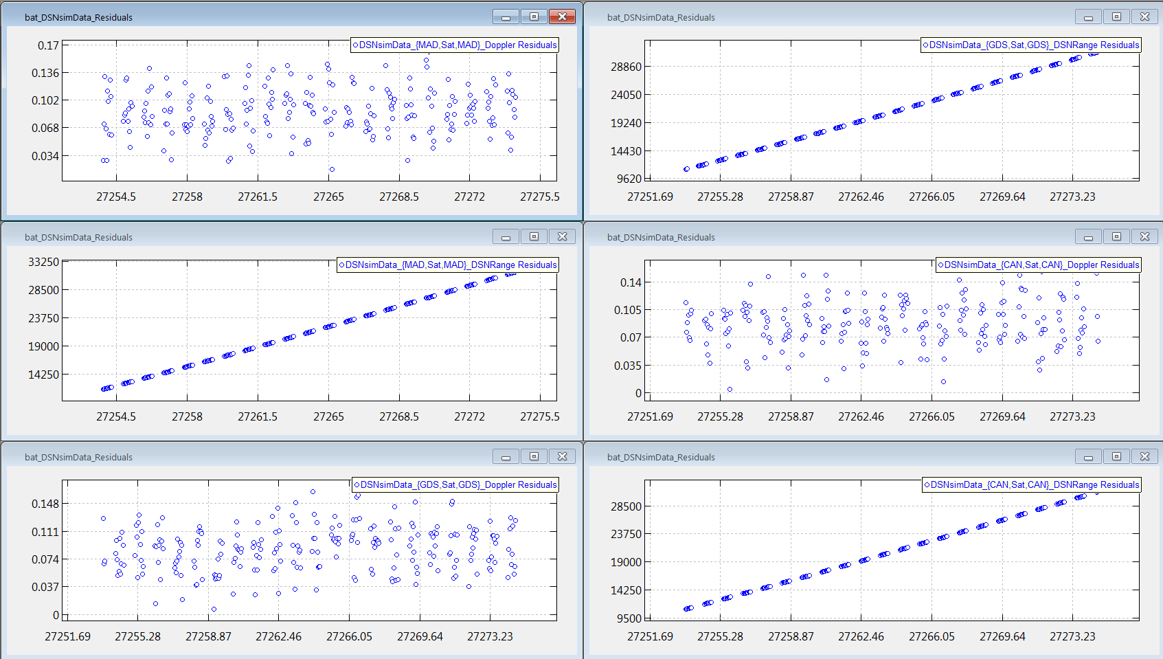
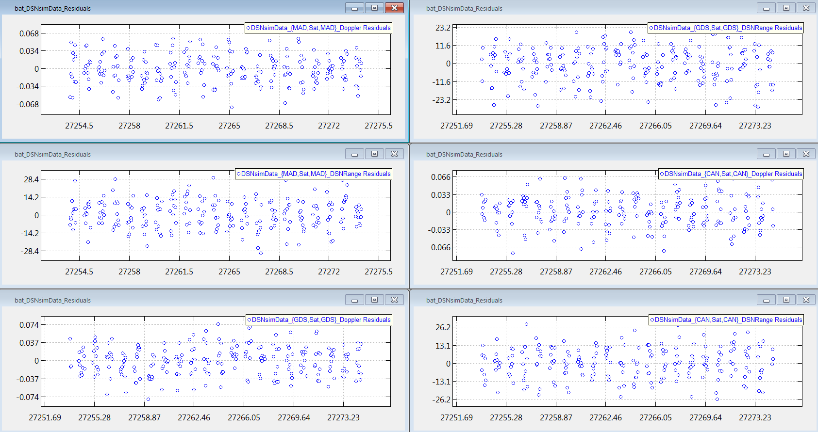
GMAT creates plots on a per iteration, per ground station, and per measurement type basis. We elaborate on what this means. When the script first runs, the first plots that show up are the 0th iteration residuals. This means that when calculating the ‘O-C’ observation residual, GMAT calculates the Computed, C, value of the residual using the a priori state. As shown in Appendix B – Zeroth Iteration Plots of Observation Residuals, there are 6 of these 0th iteration residual plots. For each of the 3 stations, there is one plot of the range residuals and one plot of the Doppler residuals. After iteration 1 processing is complete, GMAT outputs the iteration 1 residuals as shown in Appendix C – First Iteration Plots of Observation Residuals. As previously mentioned, although for this script, GMAT takes two iterations to converge, the actual iteration 2 residuals are neither calculated nor plotted. DSN_Estimation_Create_and_configure_the_Ground_Station_and_related_parameters
We now analyze the CAN range and Doppler residuals. For the 0th iteration, the range residuals vary from approximately 11,000 to 31,000 RU. These residuals are this large because our a priori estimate of the state was deliberately perturbed from the truth. There are multiple indicators on this graph that indicate that GMAT has not yet converged. First, the residuals have an approximate linear structure. If you have modeled the dynamics and measurements correctly, the plots should have a random appearance with no structure. Additionally, the residuals are biased, i.e., they do not have zero mean. For a well modeled system, the mean value of the residuals should be near zero. Finally, the magnitude of the range residuals is significantly too large. Recall that in the Create and configure the Ground Station and related parameters section, we set the 1 sigma measurement noise for the CAN range measurements to 10.63 RU. Thus, for a large sample of measurements, we expect, roughly, that the vast majority of measurements will lie between the values of approximately -32 and +32 RU. Taking a look at the 1st iteration CAN range residuals, this is, approximately, what we get.
The 0th iteration CAN Doppler residuals range from approximately 0.0050 to 0.01535 Hz. As was the case for the range 0th iteration residuals, the fact that the Doppler residuals are biased indicates that GMAT has not yet converged. Recall that in the Create and configure the Ground Station and related parameters section, we set the 1 sigma measurement noise for the CAN Doppler measurements to 0.0282 Hz. Thus, for a large sample of measurements, we expect, roughly, that the vast majority of measurements will lie between the values of approximately -0.0846 and +0.0846 RU. Taking a look at the 1st iteration CAN Doppler residuals, this is, approximately, what we get.
There is one important detail on these graphs that you should be aware of. GMAT only plots the residuals for data points that are actually used to calculate the solution. Recall that for iteration 0, all 1348 of 1348 total measurements were used to calculate the orbit state, i.e., no data points were edited. Thus, if you counted up all the data points on the 6 iteration 0 plots, you would find 1348 points. The situation is different for the 1st iteration. Recall that for iteration 1, 1346 of 1348 total measurements were used to calculate the orbit state, i.e., 2 data points were edited. Thus, if you counted up all the data points on the 6 iteration 1 plots, you would find 1346 points. If you wish to generate plots that contain both non-edited and edited measurements, you will need to generate them yourself using the MATLAB output file as discussed in the Matlab Output File section.
We note that the graphs have some interactive features. Hover your mouse over the graph of interest and then right click. You will see that you have four options. You can toggle both the grid lines and the Legend on and off. You can also export the graph data to a text file, and finally, you can export the graph image to a bmp file.
When we created our BatchEstimatorInv resource, bat, in the Create and configure BatchEstimatorInv object section, we specified that the output file name would be 'Orbit Estimation using DSN Range and Doppler Data.report. Go to GMAT’s ‘output’ directory and open this file, preferably using an editor such as Notepad++ where you can easily scroll across the rows of data.
The first approximately 150 lines of the report are mainly an echo of the parameters we input into the script such as initial spacecraft state, force model, propagator settings, measurement types to be processed, etc.
After this echo of the input data, the output report contains measurement residuals associated with the initial 0th iteration. Search the file for the words, ‘ITERATION 0: MEASUREMENT RESIDUALS’ to find the location of where the relevant output begins. This output sections contains information on all of the measurements, both non-edited and edited, that can possibly be used in the estimation process. Each row of data corresponds to one measurement. For each measurement, the output tells you the following
-
Iteration Number
-
Record Number
-
Epoch in UTC Gregorian format
-
Observation type. ‘DSN_SeqRange’ corresponds to DSN sequential range and ‘DSN_TCP’ corresponds to DSN total count phase-derived Doppler.
-
Participants. For example, ‘22222,11111,22222’ tells you that your measurement comes from a CAN to Sat to CAN link.
-
Edit Criteria.
-
Observed Value (O)
-
Computed Value (C)
-
Observation Residual (O-C)
-
Elevation Angle
We have previously discussed the edit criteria. In particular, we discussed the various reasons why data might be edited. If the edit criteria shown in the output is ‘-,’ this means that the data was not edited and the data was used, for this iteration, to calculate a state estimate.
Note that if the elevation angle of any of the measurements is below our input criteria of 7 degrees, then the measurement would be edited because the signal would be considered to be “blocked.” For range data, we would see Bn where n is an integer specifying the leg number. For our two way range data type, we have two legs, the uplink leg represented by the integer, 1, and the downlink leg, represented by the integer 2. Thus, if we saw “B1” in this field, this would mean that the signal was blocked for the uplink leg. Correspondingly, for Doppler data, we would also see Bn, but the integer n would be 1 or 2 depending upon whether the blockage occurred in the start path (n=1) or the end path (n=2).
After all of the individual iteration 0 residuals are printed out, four different iteration 0 observation summary reports, as shown below, are printed out.
-
Observation Summary by Station and Data Type
-
Observation Summary by Data Type and Station
-
Observation Summary by Station
-
Observation Summary by Data Type
After all of the observation summaries are printed out, the updated state and covariance information, obtained by processing the previous residual information, are printed out. The output also contains statistical information about how much the individual components of the state estimate have changed for this iteration.
At this point, the output content repeats itself for the next iteration. The new state estimate is used to calculate new residuals and the process starts all over again. The process stops when the estimator has either converged or diverged.
We now give an example of how this report can be used. In the Message Window Output section, we noted that, for iteration 1, two measurements were edited because of the OLSE criteria. Let’s investigate this in more detail. What type of data was edited? From what station? Could there be a problem with this data type at this station? We look at the ‘Observation Summary by Station and Data Type’ for iteration 1. We see that one range measurement from the GDS station and one range measurement from the MAD station was edited. The mean residual and 1 sigma standard deviation for GDS range measurements was -0.828187 and 10.595392 RU, respectively. The mean residual and 1 sigma standard deviation for MAD range measurements was 0.976758 and 11.047855 RU, respectively.
Now that we know that the issue was with GDS and MAD range measurements, we look at the detailed residual output, for iteration 1, to determine the time these measurements occurred. We can search for the OLSE keyword to help do this. We determine that a GDS range measurement was edited at 07 Sep 2015 19:00:00.000 UTCG and that it had an observation residual of -32.432373 RU. This is just a bit beyond the 3 sigma value and we conclude that there is no real problem with the GDS range measurements. This is just normal statistical variation.
We also determine that a MAD range measurement was edited at 31 Aug 2015 11:00:00.000 UTCG and that it had an observation residual of -33.497559 RU. Again, this is just a bit beyond the 3 sigma value and we conclude that there is no real problem with the MAD range measurements. We remind you, that when you do your run, you may have a different number of data points edited. This is because, when you do your simulation, GMAT uses a random number generator and you will be using a different data set.
In the Create and configure BatchEstimatorInv object section, when we created our
BatchEstimatorInv resource, bat, we chose our
MATLAB output file name, 'Orbit Estimation using DSN Range and
Doppler Data.mat.' By default, this file is created in GMAT’s
‘output’ directory. This file will only be created if you have MATLAB
installed and properly configured for use with GMAT.
Start up a MATLAB session. Change the directory to your GMAT ‘output’ directory and then type the following at the MATLAB command prompt.
>> load 'Orbit Estimation using DSN Range and Doppler Data.mat'
After the file has loaded, type the following command to obtain a list of available variable names inside this file.
>> whos
You should see something similar to the following:
>> whos
  Name            Size             Bytes  Class     Attributes

  Iteration0      1x1             847660  struct
  Iteration1      1x1             847690  struct
  Iteration2      1x1             847696  struct
You may see more or fewer iterations depending on your run. Each iteration variable is a structure containing the following arrays:
| Status | Observation status flag, 1 = observation is good/useable |
| IterationNumber | The iteration number. This matches the iteration number in the structure name. |
| Epoch | The TAIModJulian time tag of each observation, computed value, and residual |
| Observed | The observed value (from the GMD file) in Range Units or Hertz |
| Calculated | The predicted observation, in Range Units or Hertz, computed by GMAT using the force modeling specified in the batch estimator propagator |
| ObsMinusCalculated | The observation residual, in Range Units or Hertz |
| Elevation | The computed elevation of the observation, in degrees |
| Frequency | The transmit frequency at the time of the observation, in Hertz |
| FrequencyBand | The frequency band of the observation. See the TrackingFileSet help for a list of frequency band indicators. |
| DopplerCountInterval | The Doppler count interval in seconds, for Doppler observations. Set to -1 for range observations. |
| Participants | For each observation, a comma-separated string identifying the transmit station, tracked object, and receive station in order |
| Type | A string identifying the observation type, DSN_SeqRange or DSN_TCP |
| UTCGregorian | The UTCGregorian epoch string of each observation |
| ObsEditFlag | The editing status flag for each observation. N = not edited, U = no computed value configuration available, R = out of ramp table range, B = blocked by elevation edit criteria, IRMS = initial RMS sigma edit, OLSE = outer-loop sigma edit |
Any unset or uncomputed values are set to -1. You can use these arrays to perform custom plots and statistical analysis using MATLAB. For example, to produce a plot of all range residuals from the final iteration, you can do the following:
>> I = find(strcmp(Iteration2.Type, 'DSN_SeqRange'));
>> plot(Iteration2.Epoch(I), Iteration2.ObsMinusCalc(I), 'go');
| GTDS [1989] | Goddard Trajectory Mathematical Theory, Revision 1, Edited by A. Long, J. Cappellari, et al., Computer Sciences Corporation, FDD, FDD-552-89-0001, July 1989. |
| GTDS [2007] | Goddard Trajectory Determination System User’s Guide, National Aeronautics and Space Administration, GSFC, Greenbelt, MD, MOMS-FD-UG-0346, July 2007 |
| Moyer [2000] | Moyer, Theodore D., Formulation for Observed and Computed Values of Deep Space Network Data Types for Navigation (JPL Publication 00-7), Jet Propulsion Laboratory, California Institute of Technology, October 2000. |
| Tapley [2004] | Tapley, Schutz, Born, Statistical Orbit Determination, Elsevier, 2004 |
Running mission...

Data file 'Simulate DSN Range and Doppler Data 3 weeks.gmd' has 1348
of 1348 records used for estimation.
Total number of load records : 1348

List of tracking configurations (present in participant ID) for load
records from data file
'Simulate DSN Range and Doppler Data 3 weeks.gmd':

   Config 0: {{22222,11111,22222},DSN_SeqRange}
   Config 1: {{22222,11111,22222},DSN_TCP}
   Config 2: {{33333,11111,33333},DSN_SeqRange}
   Config 3: {{33333,11111,33333},DSN_TCP}
   Config 4: {{44444,11111,44444},DSN_SeqRange}
   Config 5: {{44444,11111,44444},DSN_TCP}


****   No tracking configuration was generated because the tracking
configuration is defined in the script.
********************************************************
*** Performing Estimation (using "bat")
***
********************************************************

a priori state:
   Estimation Epoch:
       27253.500417064603 A.1 modified Julian
       27253.500416666666 TAI modified Julian
   19 Aug 2015 00:00:00.000 UTCG
   Sat.SunMJ2000Eq.X = -126544963
   Sat.SunMJ2000Eq.Y = 61978518
   Sat.SunMJ2000Eq.Z = 24133225
   Sat.SunMJ2000Eq.VX = -13.789
   Sat.SunMJ2000Eq.VY = -24.673
   Sat.SunMJ2000Eq.VZ = -10.662

Number of Records Removed Due To:
   . No Computed Value Configuration Available : 0
   . Out of Ramp Table Range   : 0
   . Signal Blocked : 0
   . Initial RMS Sigma Filter  : 0
   . Outer-Loop Sigma Editor : 0
Number of records used for estimation: 1348

   WeightedRMS residuals for this iteration : 1459.94235975
   BestRMS residuals for this iteration     : 1459.94235975
   PredictedRMS residuals for next iteration: 1.01539521333

------------------------------------------------------
Iteration 1

Current estimated state:
   Estimation Epoch:
       27253.500417064603 A.1 modified Julian
       27253.500416666666 TAI modified Julian
   19 Aug 2015 00:00:00.000 UTCG
   Sat.SunMJ2000Eq.X = -126544968.377
   Sat.SunMJ2000Eq.Y = 61978514.8777
   Sat.SunMJ2000Eq.Z = 24133217.2547
   Sat.SunMJ2000Eq.VX = -13.7889998632
   Sat.SunMJ2000Eq.VY = -24.6730006664
   Sat.SunMJ2000Eq.VZ = -10.6619986007

Number of Records Removed Due To:
   . No Computed Value Configuration Available : 0
   . Out of Ramp Table Range                   : 0
   . Signal Blocked                            : 0
   . Initial RMS Sigma Filter                  : 0
   . Outer-Loop Sigma Editor                   : 2
Number of records used for estimation          :1346

   WeightedRMS residuals for this iteration : 1.00807187051
   BestRMS residuals for this iteration     : 1.00807187051
   PredictedRMS residuals for next iteration: 1.00804237273
This iteration is converged due to relative convergence criteria.


********************************************************
*** Estimating Completed in 2 iterations
********************************************************

Estimation converged!
      |1 - RMSP/RMSB| = | 1- 1.00804 / 1.00807| = 2.92616e-005 is
	  less than RelativeTol, 0.0001

Final Estimated State:

   Estimation Epoch:
       27253.500417064603 A.1 modified Julian
       27253.500416666666 TAI modified Julian
   19 Aug 2015 00:00:00.000 UTCG
   Sat.SunMJ2000Eq.X = -126544968.759
   Sat.SunMJ2000Eq.Y = 61978514.3889
   Sat.SunMJ2000Eq.Z = 24133216.7847
   Sat.SunMJ2000Eq.VX = -13.7889997238
   Sat.SunMJ2000Eq.VY = -24.673000621
   Sat.SunMJ2000Eq.VZ = -10.6619988668
Final Covariance Matrix:

        6.566855211518e+000        1.044634165793e+001        3.112863356104e+000       -2.345908150453e-006        5.035500518048e-007        1.602400702334e-006
        1.044634082751e+001        2.043155461343e+001       -4.258301029878e+000       -3.704075903144e-006        2.022938490903e-007        3.971535902921e-006
        3.112865361595e+000       -4.258297445960e+000        2.371732979013e+001       -1.178974996784e-006        1.683977194948e-006       -2.674173473312e-006
       -2.345908159193e-006       -3.704076213842e-006       -1.178974284159e-006        8.386165742100e-013       -1.658563839962e-013       -6.047842793431e-013
        5.035500497713e-007        2.022939026968e-007        1.683977056710e-006       -1.658563826712e-013        1.032575255469e-012       -2.190676053421e-012
        1.602400700119e-006        3.971536117909e-006       -2.674174002075e-006       -6.047842762516e-013       -2.190676053038e-012        5.776276322091e-012

Final Correlation Matrix:

             1.000000000000             0.901851016006             0.249429858518            -0.999655967713             0.193376220513             0.260176714954
             0.901850944314             1.000000000000            -0.193442883328            -0.894844247176             0.044042413976             0.365581159741
             0.249430019216            -0.193442720520             1.000000000000            -0.264356490609             0.340284723675            -0.228471850851
            -0.999655971438            -0.894844322236            -0.264356330820             1.000000000000            -0.178233614796            -0.274786120507
             0.193376219732             0.044042425647             0.340284695741            -0.178233613372             1.000000000000            -0.897001819395
             0.260176714594             0.365581179531            -0.228471896026            -0.274786119102            -0.897001819239             1.000000000000

********************************************************


Mission run completed.
===> Total Run Time: 85.739000 seconds

========================================