Recursive Model Estimation Methods (System Identification Toolkit)
Recursive model estimation is a system identification technique that enables you to develop a model that adjusts based on real-time data coming from the system. Recursive model estimation processes the measured input-output data recursively as the data becomes available. This technique is helpful because you obtain the mathematical model of the system in real time. In many real-world applications such as adaptive control and adaptive prediction, having a model of the system update while the system is running is necessary or helpful.
By comparison, the nonparametric, parametric, partially known, and closed-loop systems model estimation methods use nonrecursive methods to estimate a model of the plant in a system. These nonrecursive methods identify a model for a plant based on input-output data gathered at a time prior to the current time.
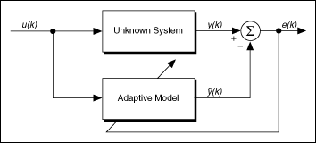
The following figure represents a general recursive system identification application. A system identification application consists of an unknown system that has an input signal, or stimulus signal u(k) and an output signal, or response signal y(k).

The stimulus signal u(k) is the input to both the unknown system and the recursive model. The response of the system y(k) and the predicted response of the adaptive model  are combined to determine the error of the system. The error of the system is defined by the following equation.

The adaptive model generates the predicted response  based on u(k + 1) after adjusting the parametric vector
  based on the error e(k).
The previous figure shows how the error information e(k) is sent back to the adaptive model, which adjusts the parametric vector  to account for the error. You iterate on this process until you minimize the magnitude of the least mean square error e(k).
Before you apply the recursive model estimation, you must first select the parametric model structure that determines the parametric vector  . Then, you must select the method that automatically adjusts the parametric vector such that the error e(k) goes to the minimum.
The LabVIEW System Identification Toolkit provides Recursive Model Estimation VIs, which you can use to estimate the following parametric model representations:
Refer to the Online Model Estimation VI in the labview\examples\System Identification\Getting Started\Recursive Estimation.llb for an example that demonstrates how to use the SI Recursively Model Estimation VIs to estimate the linear models for an unknown system recursively.
 Open example
 Browse related examples
The Recursive Model Estimation VIs have a recursive method parameter that enables you to specify which recursive estimation method to use. The adaptive method you use affects the performance of recursive system identification application. You can choose from the following four methods:
- Least mean squares (LMS)
- Normalized least mean squares (NLMS)
- Recursive least squares (RLS)
- Kalman filter (KF)
The goal of each method is to adjust the parametric vector  until you minimize the cost function J(k). The following equation defines the cost function J(k).
J(k) = E[e 2(k)]
where E is the expectation of the enclosed term(s).
When the cost function J(k) is sufficiently small, the parametric vector  is considered optimal for the estimation of the actual system.