Partially Known Model Estimation Case Study (System Identification Toolkit)

This case study gives an example that uses the prior knowledge you have about a system to define and estimate state-space models. You use the same procedure when estimating continuous transfer function models. However, you apply different methods to define continuous transfer function models.

The following figure shows an RLC circuit, where u is the input voltage, y is the output voltage, i_L is the current, and u_C is the capacitor voltage. In this example, y equals the capacitor voltage u_C.

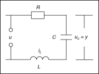
Suppose R is 1.5 Ω and L and C are unknown. You can complete the following steps to identify the values of L and C.

1. Apply a wide-band voltage to u and measure the output y simultaneously. The Continuous State-Space Model of an RLC Circuit example VI uses a chirp signal from 0.5 Hz to 6 Hz as the stimulus signal. The response to the chirp signal is the response signal. This example VI then preprocesses the stimulus and response signals to remove the offset level in these signals.
2. Define a model for this circuit. Because you have information about the approximate values of L and C, you can build a partially known state-space model or a partially known transfer function model.
3. Estimate the model you defined in step 2 and then estimate L and C.

The Continuous State-Space Model of an RLC Circuit example VI guides you through defining and estimating a state-space model for the RLC circuit.

Refer to the Continuous State-Space Model of an RLC Circuit VI in the labview\examples\System Identification\Getting Started\Grey-Box Model.llb to access the VI in this case study.

Open example  Browse related examples

Refer to the Continuous Transfer Function Model of a DC Motor with Known Gain VI in the labview\examples\System Identification\Getting Started\Grey-Box Model.llb for an example that demonstrates how to use a partially known transfer function model to estimate the RLC circuit.

Open example  Browse related examples

You can use the following first-order differential equation to represent the relationship between the capacitor voltage and the current of this RLC circuit.

You can use the following first-order differential equation to represent the voltage relationship in this RLC circuit.

By manipulating the previous two equations, you can deduce the continuous state-space model for this RLC circuit using the following two equations:

The LabVIEW System Identification Toolkit provides the SI Create Partially Known State-Space Model VI with which you can build the symbolic state-space model for this circuit, as shown in the following figure.

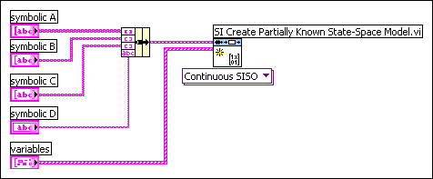
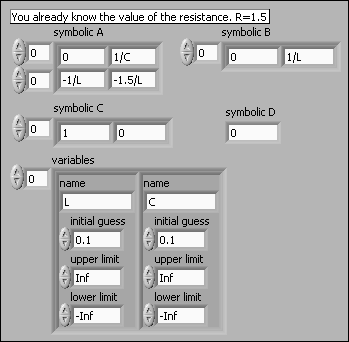
You specify the symbolic state-space model using formula strings, such as 1/C, -1/L, and -1.5/L, with L and C as variables. Then you define L and C with the variables input, as shown in the following figure. Using prior knowledge, you know that L is a positive value around the initial value of 0.1 H, and C is a value between 0 F and 0.3 F.

Next, you can estimate the state-space model with the SI Estimate Partially Known State-Space Model VI, as shown in the following figure.

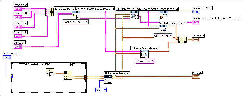
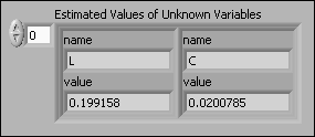
The SI Estimate Partially Known State-Space Model VI estimates each parameter of the model. You obtain the estimated model and optimized variables of the model after this VI performs an optimization. In this example, you obtain the values 0.20 H for L and 0.02 F for C, as shown in the following figure.

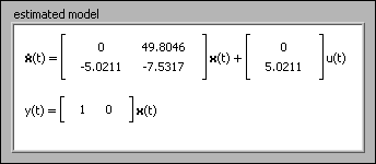
The Continuous State-Space Model of an RLC Circuit example VI uses the SI Draw Model VI and the values of L and C you obtain to display the estimated model in a picture indicator, as shown in the following figure.

You then can determine how accurately this model simulates the real-world plant by validating the model. Refer to the System Identification Case Study book for an example of validating a model.