State-Space Model Definitions (System Identification Toolkit)

The state-space model is the most convenient model for describing multiple-input multiple-output (MIMO) systems. State-space models often are preferable to polynomial models, especially in modern control applications that focus on multivariable systems. You can estimate both continuous and discrete state-space models.

Continuous

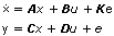
Use partially known model estimation methods to estimate continuous state-space models. You must provide an initial guess for each parameter before conducting estimation. The following equations show the form of the continuous state-space model.

Discrete

Use the SI Estimate State-Space Model and SI Estimate State-Space Model from FRF VIs to estimate discrete state-space models. The SI Estimate State-Space Model VI supports the following two estimation methods:

• Deterministic-stochastic subspace method—This method uses principal component analysis to estimate parameters. This method uses both stimulus and response signals to estimate state-space models. This method includes the stochastic parts of the system in the model structure.
• Realization method—This method uses the impulse response to estimate only the deterministic state-space model. This method does not include stochastic parts of the system in the model structure.

Refer to the LabVIEW System Identification Toolkit Algorithm References manual for more information about the deterministic-stochastic subspace method and the realization method.

The following equations show the form of the discrete state-space model.

x(k + 1) = Ax(k) + Bu(k) + Ke(k)

y(k) = Cx(k) + Du(k) + e(k)

Note  The equations for the discrete state-space model based on frequency-domain data do not contain Ke(k) and e(k).

where	A is an n × n state matrix of the given system
	B is an n × m input matrix of the given system
	C is an r × n output matrix of the given system
	D is an r × m direct transmission matrix of the given system
	K is the Kalman gain matrix
	k is the model sampling time multiplied by the discrete time step, where the discrete time step equals 0, 1, 2, …
	n is the number of model states
	m is the number of model inputs
	r is the number of model outputs
	x is the model state vector
	u is the model input vector
	y is the model output vector
	e(k) is the system disturbance

The state-space transfer matrices A, B, C, and D often reflect physical characteristics of a system. The dimension of the state vector x is the only setting you must provide for the state-space model.