General-Linear Model Definitions (System Identification Toolkit)

Generally, you can describe a discrete system by using the general-linear polynomial model. This model provides flexibility for both system dynamics and stochastic dynamics.

Use the SI Estimate General Linear Model VI to estimate general-linear polynomial models. The following equation describes this model.

y(k) = z ^–n G(z ^–1, θ)u(k) + H(z ^–1, θ)e(k)

where	u(k) and y(k) are the input and output of the system, respectively
	e(k) is the disturbance of the system which usually is zero-mean white noise
	G(z–1, θ) is the transfer function of the deterministic part of the system
	H(z–1, θ) is the transfer function of the stochastic part of the system

The deterministic transfer function specifies the relationship between the output and the input signal. The stochastic transfer function specifies how the random disturbance affects the output signal. Often the deterministic and stochastic parts of a system are referred to as system dynamics and stochastic dynamics, respectively.

The term z ^–1 is the backward shift operator, which is defined by the following equations:

z ^–1 x(k) = x(k - 1)

z ^–2 x(k) = x(k - 2)

...

z ^–n x(k) = x(k - n)

z ^–n defines the number of delay samples between the input and the output.

G(z ^–1, θ)u(k) and H(z ^–1, θ)e(k) are rational polynomials as defined by the following equations:

The vector θ is the set of model parameters. The following equations do not display θ to make the equations easier to read.

The following equation shows the form of the general-linear model.

where	y(k) is the system outputs
	u(k) is the system inputs
	n is the system delay
	e(k) is the system disturbance

A(z), B(z), C(z), D(z), and F(z) are polynomial with respect to the backward shift operator z ^-1 and defined by the following equations.

The following figure depicts the signal flow of a general-linear model.

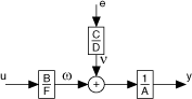
where	u is the system inputs
	e is the system disturbance
	y is the system outputs

Setting one or more of A(z), C(z), D(z), and F(z) equal to 1 can create simpler models such as autoregressive with exogenous terms (ARX), autoregressive-moving average with exogenous terms (ARMAX), output-error, and Box-Jenkins models, which you commonly use in real-world applications.

SISO

The following are the time domain equations for the general-linear SISO model.

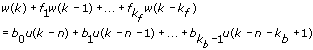
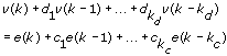
where	kf is the F order
	kb is the B order
	kc is the C order
	kd is the D order
	ka is the A order
	u(k) is the system inputs
	n is the system delay
	e(k) is the system disturbance

Refer to the Estimate Polynomial Models VI in the labview\examples\System Identification\Getting Started\Parametric Estimation.llb for an example that demonstrates how to estimate general-linear polynomial models for an unknown system.

Open example  Browse related examples