Frequency-Domain Model Estimation Case Study (System Identification Toolkit)

This case study demonstrates how to use frequency-domain data from a flexible robotic arm to estimate and validate a transfer function model and state-space model of the robotic arm. This case study estimates the models directly from frequency-domain data.

Note  If the system you want to estimate contains time-domain data, you first must estimate the FRF by using the SI Estimate FRF VI.

Refer to the Flexible Arm (Frequency Domain) VI in the labview\examples\System Identification\Industry Applications\Mechanical Systems.llb to access the VI in this case study.

Open example  Browse related examples

In this case study, the input is voltage and the outputs are strain and position. Strain is proportional to the acceleration of the flexible arm. Position is the radial position of the arm.

Because this system contains one input and two outputs, two single-input single-output (SISO) FRFs or one multiple-input multiple-output (MIMO) FRF define this system. One FRF defines the relationship between the voltage input and the strain output. The other FRF defines the relationship between the voltage input and the position output. Each FRF contains information about the magnitude and phase of the frequency response and the scale of the frequency data. This information is specific to each input-output pair. To measure the FRFs in this case study, sine waves at different frequencies excite the flexible arm. This data set has a sampling time of 0.02 seconds, which is equivalent to a sampling rate of 50 Hz.

Estimating and Validating a Transfer Function Model

Use the SI Estimate Transfer Function Model from FRF VI to estimate a transfer function model from a SISO FRF. Because this case study involves one input and two outputs, this VI must estimate and validate each SISO transfer function model separately. The following figure shows the block diagram for estimating a transfer function model and validating the resulting transfer function model against the original FRF data. This block diagram uses the FRF describing the relationship between the voltage input and the position output to estimate the transfer function model.

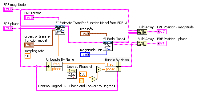
The FRF magnitude and the FRF phase inputs of the SI Estimate Transfer Function Model from FRF VI require that the data input is in polar form.

Note  If the data input is in complex form, you can use the Re/Im To Polar Function to convert the complex data into polar form to separate the magnitude, phase, and frequency components of the complex representation. After converting the complex data into polar form, bundle the magnitude and frequency components into one cluster and bundle the phase and frequency components into another cluster. Each cluster then contains the data you wire to the FRF magnitude and the FRF phase inputs of the SI Estimate Transfer Function Model from FRF VI.

In this case study, the FRF magnitude and the FRF phase inputs contain data in polar form. Therefore, the FRF magnitude and the FRF phase inputs wire directly into the SI Estimate Transfer Function Model from FRF VI.

Note  The FRF format input of this VI specifies whether the original FRF magnitude is in decibels or in a linear scale and whether the original FRF phase is wrapped and in radians or in degrees. In this case study, the original FRF data uses the default values of FRF format. The original FRF magnitude is not in decibels. The original FRF phase is wrapped and in radians.

Because a transfer function model is a type of parametric model representation, you must specify the model parameters before estimating the model. For a transfer function model, you must specify the orders of the numerator and denominator polynomial functions. If you do not have prior knowledge about the system, you must use trial and error to determine the optimal orders of the model.

One way to identify the optimal orders is to observe the peaks in the magnitude response of the original FRF. The optimal order is at least twice the number of peaks. You can plot and observe the magnitude by using the SI Bode Plot VI. You can increase the accuracy of the model by modifying the initial guess after analyzing the model. In the previous block diagram, 2 is the initial guess for both the numerator order and the denominator order.

You can validate the resulting model by comparing the original FRF and the FRF that the model generates. Compare the two FRFs on an XY graph by using the SI Bode Plot VI. By default, the SI Bode Plot VI unwraps the phase information and converts the units of the resulting phase to degrees. To compare the original FRF and the FRF that the SI Bode Plot VI displays more accurately, use the Unwrap Phase VI to unwrap the phase in the original FRF. This case study also uses the Mathematics VIs to convert the original FRF from radians to degrees.

The following figure shows the Bode plot of a 2nd-order transfer function model.

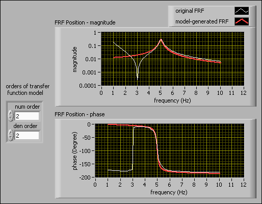
Visually inspect the alignment of the model-generated FRF and the original FRF to determine whether the estimated transfer function model accurately describes the plant. Notice that the original FRF and the model-generated FRF do not align at frequencies lower than 4 Hz. Therefore, 2 is not the most appropriate order value for the transfer function model.

You can increase the accuracy of the model by specifying different values for the orders of transfer function model control. The following figure shows the Bode plots of a 6th-order transfer function model.

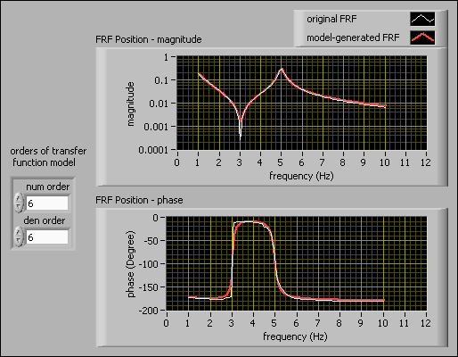
In this case study, setting the value of the orders of transfer function model to 6 provides a closer alignment of the model-generated FRF and the original FRF. Therefore, a 6th-order transfer function model describes the voltage-position FRF of the plant more accurately than a 2nd-order model.

Identify a second transfer function model by using the FRF of the voltage input and strain output. You must apply the same method when optimizing the model order.

Estimating and Validating a State-Space Model

In this case study, a single MIMO FRF also can represent the frequency-domain relationship of the input and outputs of the flexible arm system. You can use this MIMO FRF to estimate state-space models of a plant. The SI Estimate State-Space Model from FRF VI estimates a state-space model for SISO and MIMO systems. This VI requires you to specify the number of states of the system you want to estimate. This value comes from prior knowledge about the system.

You also can provide an initial guess if you do not have prior knowledge. A guideline for identifying the number of states of a system is the same as the guideline for identifying the orders of a transfer function model. The number of states is at least twice the number of peaks in the magnitude of the FRF. Because a MIMO FRF is composed of more than one SISO FRF, you must observe the magnitude of the SISO FRF with the maximum number of peaks.

In this case study, the SISO FRFs that comprise the MIMO FRF both have one peak. Therefore, the initial guess at the number of states is 2. By increasing the number of states and plotting the model-generated MIMO FRF along with the original MIMO FRF on a Bode plot, you can observe that entering eight states produces an acceptable estimation for the system.

The following figure shows the Bode Plots of the original MIMO FRF and the MIMO FRF that the state-space model generates.

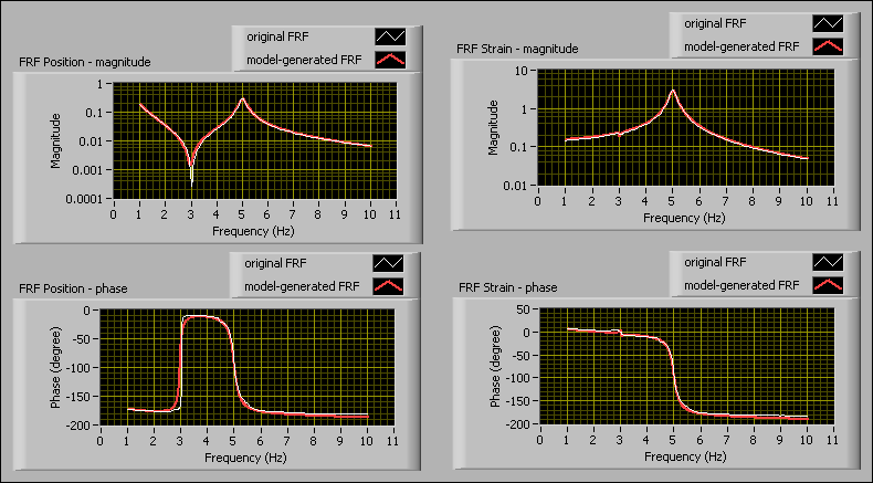
Compare the FRF Position graphs in the previous figure with the 6th-order transfer function FRF Position graphs. Both model-generated FRFs are close to the original FRF in the FRF Position graphs. The proximity of these FRFs indicates that the 6th-order transfer function model and the state-space model with eight states are close approximations for estimating system models in this case study.