Analyzing Models (System Identification Toolkit)

You can use model analysis to observe some characteristics, such as frequency response, stability, and order, of the model. Use the LabVIEW System Identification Toolkit to investigate model estimation results and present these results in Bode plot, the Nyquist plot, and the pole-zero plot graphs.

Refer to the Model Presentation VI in the labview\examples\System Identification\Getting Started\General.llb for an example that demonstrates how to use the SI Bode Plot, SI Nyquist Plot, and SI Pole-Zero Plot VIs to compute the Bode, Nyquist, and pole-zero plots, respectively, of an system model.

Bode Plot

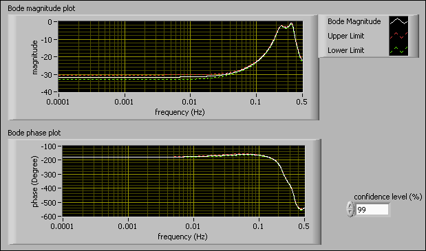
A Bode plot contains a Bode magnitude plot and a Bode phase plot. These two plots together describe the frequency response of the plant model you estimate. A Bode magnitude plot describes magnitude versus frequency. A Bode phase plot describes phase versus frequency. The following figure shows an example of a Bode plot.

The SI Bode Plot VI calculates the upper and lower limits according to the confidence level you set. You can obtain information, such as the gain of the system and the cutoff frequency, by evaluating the Bode plot. You can use the SI Bode Plot VI to produce the Bode magnitude and Bode phase plots. You then can display the Bode magnitude and phase using the SI Bode Plot Indicator.

Nyquist Plot

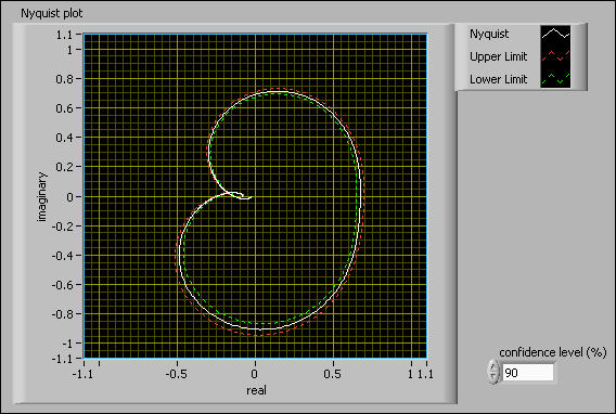
A Nyquist plot describes the gain and phase of a frequency response in polar coordinates by plotting the imaginary part of the complex frequency response versus the real part. You can use the Nyquist plot to predict the stability of a system. In polar coordinates, a Nyquist plot shows the phase as the angle and the magnitude as the distance from the origin, as shown in the following figure.

The SI Nyquist Plot VI calculates the upper and lower limits according to the confidence level you set. You can use the SI Nyquist Plot VI to generate the Nyquist plot and display this plot by using the SI Nyquist Plot Indicator.

Pole-Zero Plot

The pole-zero plot displays the poles and zeros of a system. By observing the locations of the poles and zeros, you can conclude whether the system is stable. In a stable system, all poles are within the unit circle. The following figure shows a pole-zero plot of a stable model.

You can use the SI Pole-Zero Plot VI to generate a pole-zero plot and display the plot by using the SI Pole-Zero Plot Indicator.

You also can use the pole-zero plot to determine if you can reduce model orders. By observing the pole-zero placements, you can determine if any pole-zero pairs have overlapping confidence intervals. A confidence interval is a region the SI Pole-Zero Plot VI calculates from the confidence level you set. The existence of overlapping confidence intervals implies that pole-zero cancellations exist and that the model order might be unnecessarily high. The pole-zero plot shown in the previous figure is an optimal model with the appropriate order because the pole-zero pairs do not have overlapping confidence intervals.

If the model order is too high, you can try reducing the model order. You then can use the F-test criterion to assess if the reduction in model order leads to a significant increase in the prediction error. If the reduction in model order leads to a significant increase in the prediction error, do not reduce the model order.