Applying a Lag Window (System Identification Toolkit)

When computing Φ_uu(e^jω) and Φ_uy(e^jω) to obtain the frequency response G(e^jω), you can apply a lag window ω(τ) to the autocorrelation function R_uu and the cross-correlation function R_uy before performing the FFT operation. Applying a lag window improves the accuracy of the frequency response estimation, according to the following equations.

The lag window approaches zero when the lag τ is large. The window weighs out the points of R_uu and R_uy with large lag τ, thereby improving the accuracy of the frequency response estimation. The SI Estimate Frequency Response VI uses a Hanning window as the lag window.

The frequency response with the lag window, G'(e^jω), is equivalent to the moving average version of the frequency response without the lag window, G(e^jω). The average smooths the frequency response, but the smooth frequency response also can deviate from the true frequency response. Adjusting the length of the lag window can balance the trade-off between variance and bias of the frequency response estimation. The larger the length of the lag window, the fewer points of G(e^jω) the SI Estimate Frequency Response VI averages to compute G'(e^jω), and hence the larger the variance and the smaller the bias of the frequency estimation.

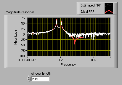
The following example demonstrates how the length of the lag window affects the frequency response estimation. The following figure shows the front panel of a VI that simulates a system defined by the following equation.

y(k) – 1.46y(k – 1) + 2.5y(k – 2) – 1.46y(k – 3) + yk – 4 = u(k) + 0.45u(k – 1) + u(k – 2)

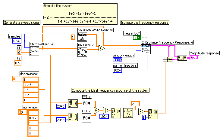
The following figure shows the block diagram of this VI.

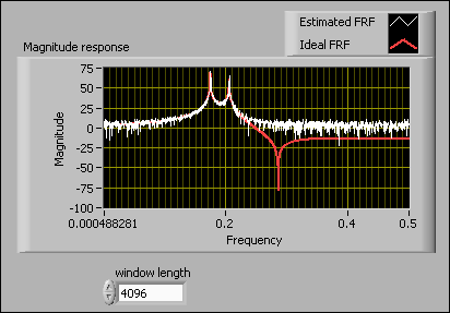
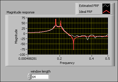
In this example VI, the input signal u(k) is a swept sine wave whose normalized frequency is from 0 to 0.5 Hz. The number of data points in the input signal is 4096. The length of the lag window therefore must be less than or equal to 4096. The following figures show the resulting frequency responses when the window length is 4096 and 64, respectively.

The frequency response curve is smoother and the variance is smaller when the length of the lag window is small. However, when the length of the lag window is too small, you cannot distinguish between the two close peaks in the frequency response, as shown in the previous figure with window length equal to 64. When the length of the lag window is large, the SI Estimate Frequency Response VI accurately estimates the peaks, as shown in the previous figure with window length equal to 4096. The bias is small with a large lag window, but the variance of the estimated frequency response is large.

Setting the length of the lag window to 5–10% of the number of data points when estimating the frequency response often results in a good trade-off between the bias and variance. The length also depends on the signals, the properties of the system, and the purpose of application. For example, to identify the passband of a system, use a smaller lag window. To identify the dynamic properties of a system, such as its natural frequency, use a larger lag window.