Preprocessing the Data (System Identification Toolkit)
After you gather data, the next step in the system identification process is to preprocess the data. The input to the system in this case study is the reaction torque of the structure on the ground. This input is a swept sine wave with 200 frequency points equally spaced over the frequency band from 0.122 Hz to 24.4 Hz.
The output of this system is the acceleration of the flexible arm. The acceleration contains information about the flexible resonances and anti-resonances.
The data set contains 4096 samples at a sampling rate of 500 Hz or sampling time of 0.002 seconds. Thus the total time of the response is 8.192 seconds.
You can preprocess the raw data by examining the time and frequency responses of the system. Based on those analyses, you can filter and downsample the data set to reduce the amount of data in the raw data set for simpler identification.
Examining the Time Response Data
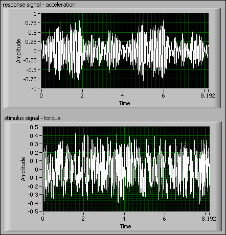
Using the data in the SI Data Samples VI for the flexible robotic arm, you can view the input and output data, as shown in the following figure.

The stimulus signal – torque output corresponds to the input data, or the torque, and the response signal – acceleration output corresponds to the output data, or the acceleration.
The following figure shows the input and output data on graphs during the length of the response. By looking at the graphs, you can inspect the data for outliers, clipped saturation, or quantization effects that you can remove because they are not representative of the system behavior.

The previous figure shows no obvious nominal, trend, or outlier values in the input or output time waveforms.
Examining the Frequency Response Data
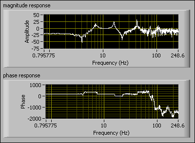
In addition to examining the time response data, you also want to examine the frequency response data. You can use the SI Estimate Frequency Response VI to view the frequency response of the measured output signal, as shown in the following figure.

The input data is periodic over 4096 samples, which is the signal length. Notice that in the previous figure the window length, 4096, is the same as the signal length so as to obtain a smaller bias in the frequency response estimation.
The following figure shows the magnitude and phase responses of the measured output signal. The magnitude response graph shows three resonances and two anti-resonances in the frequency domain. Resonances are vibrations of large amplitude in a system caused by exciting the system at its natural frequency.

Notice the resonance at approximately 42 Hz. You can deduce that this resonance is caused by noise or nonlinear system behavior because the 42 Hz falls outside the frequency range of the input data, 0.122–24.4 Hz. At 42 Hz, there is no input energy, thus implying that the response at 42 Hz is not a result of the input.
By examining the frequency response data, you see that filtering is necessary to remove this resonance peak at 42 Hz. You can use the LabVIEW System Identification Toolkit to apply a filter to the flexible arm data.
Applying a Filter to the Raw Data
To eliminate the resonance peak at 42 Hz, you can apply a filter to the raw data. By first applying a lowpass filter with a cutoff frequency of 25 Hz, you eliminate the high-frequency noise from the raw data set. The following figure shows how to use SI Lowpass Filter to apply a lowpass filter to the raw data set.

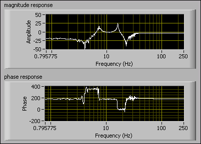
You can see the effects of the lowpass filter by comparing the frequency response of the filtered data set in the following figure to the frequency response of the non-filtered data set. By using a lowpass filter, you can see that the resonance at approximately 42 Hz is no longer part of the data set you will use to estimate the model.

Downsampling the Raw Data
Sampling theory, in conjunction with the Nyquist criterion, enables you to reduce the sampling rate from 500 Hz to 50 Hz. Applying a filter and downsampling the data set reduces the number of samples in and the computational complexity of the data set. The goal is to use as few samples as possible to evaluate the behavior of the system.
Sampling theory enables you to downsample, or decimate, the data set. Downsampling reduces the sampling rate, 500 Hz, by a factor of 10. Thus downsampling enables you to acquire the data at a sampling rate of 50 Hz. The Nyquist criterion states that you must sample the signal at a minimum of twice the highest frequency in the system.
Recall that the input data is equally spaced over the frequency band 0.122–24.4 Hz. Therefore, according to the Nyquist criterion, you must sample at a minimum of 50 Hz to avoid any antialiasing. The benefit of sampling at 50 Hz is that you still acquire all the data in the frequency band, yet you eliminate the resonance peak at 42 Hz.
Therefore, in the following figure, the SI Lowpass Filter VI sets the cutoff frequency to 25. In addition to applying a lowpass filter to the data, you must downsample the reduced data set. The SI Down Sampling VI in the following figure uses a decimation factor of 10.

The SI Lowpass Filter VI applies a lowpass filter before downsampling the data set to avoid aliasing at the 42 Hz resonance. Together, the lowpass filter and downsampling remove the high frequency disturbance and make the process faster and more efficient.
Notice that the window length parameter of the SI Estimate Frequency Response VI in the previous figure is around 400 instead of 4096, as shown in the previous figure. You can reduce the window length by a factor of 10 because the number of samples in the reduced data set is one tenth of the number of samples in the raw data set.
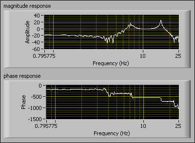
The following figure shows the frequency response after applying a filter to and downsampling the raw data set.

Filtering and downsampling are beneficial because they eliminate the nonrealistic parts of the frequency response and reduce the amount of work required in the model estimation process.