Home > Getting Started Guide > Creating a Simple Pivot Table in Excel > Pivot Tables Excel 2003 > Create a Pivot Table Report
Create a Pivot Table Report
To create a Pivot Table you need to identify these two elements in your data:
Have a list in Excel with data fields (headings) and rows of related data
Identify which fields are going to go where in your design
Method
Select any cell in the data list
On the Menu bar select Data
Select Pivot Table and Pivot Chart Wizard.
Make sure that Microsoft Excel list or database is selected as the data to analyze
Make sure the kind of report is selected as Pivot Table.
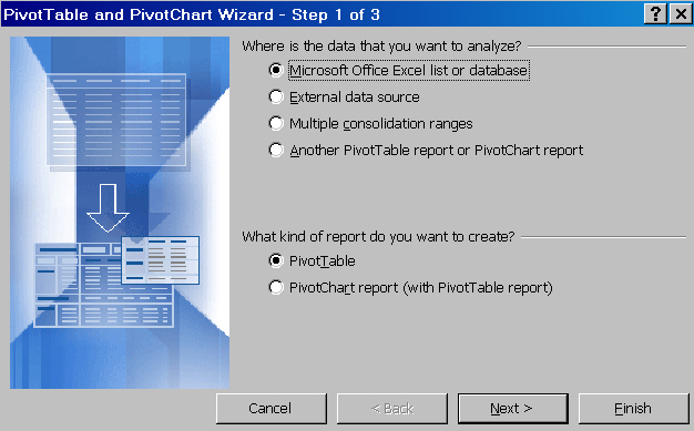
Select Next
Select the collapse icon in the range box
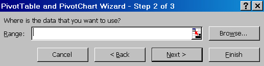
Select the data range on the worksheet that contains the source data
The selected range will appear in the range box

Select the collapse icon again to return to your active worksheet .
Select Next
On the next screen, select where you want to place the Pivot Table, select New Worksheet
Choose another cell if you do not want the current cell as the position on the worksheet
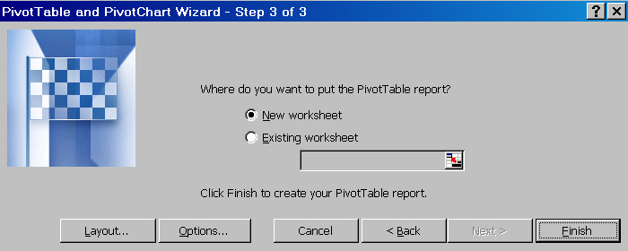
Select Layout
The Pivot Table and Pivot Chart Wizard – layout window appears
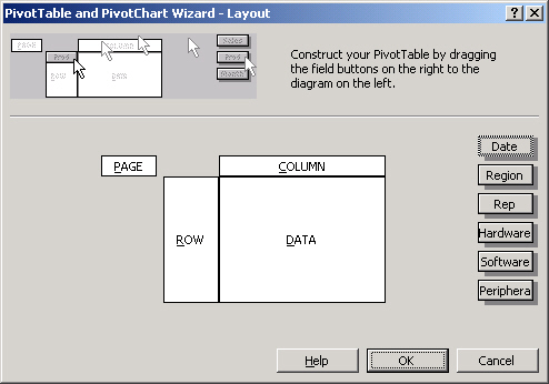
The column headings from the source data will now appear as fields on the right
Drag the fields to the relevant positions on the layout
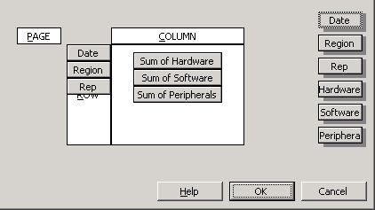
Select OK
Select Options
Select your required options
Select OK
Select Finish
The Pivot Table will be now be displayed