In this exercise, you will use the FR Paste Function screen and the FRACCT function to search a range of accounts for words appearing in the account description.

1. Select cell F10.
2. On the Add-Ins tab of the Excel ribbon, click the arrow beside FR, and then click FR Paste.
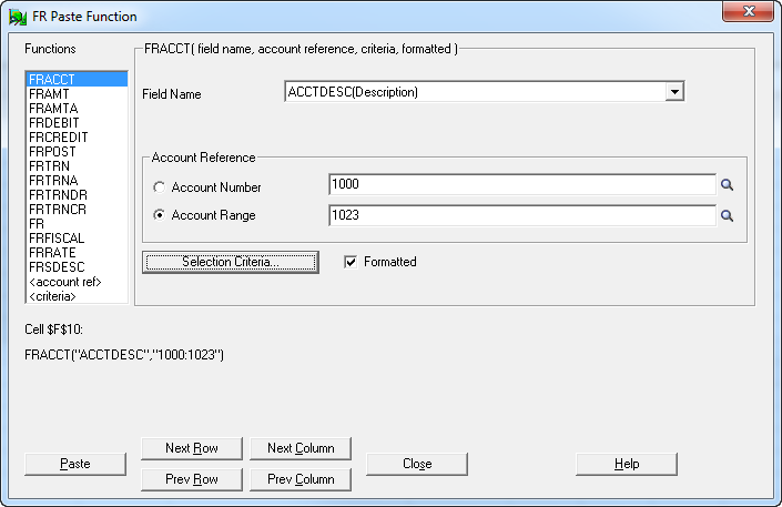
3. On the FR Paste Function screen, specify a range of account descriptions to search.
   1. On the Functions list, click FRACCT.

      The syntax for FRACCT (field name, account reference, criteria, formatted) appears to the right of the Functions list.

   2. On the Field Name list, select ACCTDESC(Description).
   3. In the Account Reference group, select the Account Range option.
   4. Specify a range of accounts.
      1. In the first field in the Account Reference group, enter 1000.
      2. In the first field in the Account Reference group, enter 1023.
   5. Leave the Formatted option selected.

   You have now created a formula that instructs Financial Reporter to scan the descriptions of every account in the range you specified, and to return any words that are common to all account descriptions in that range. (In this example, the word that appears in every account description is "Sales.")

   The formula to be pasted into the spreadsheet appears below the Functions list. Show Me.

   

4. Click the Paste button to paste the formula into cell F10.
5. Click Close to close the FR Paste Function screen.

   In the spreadsheet, the word "Sales" appears in cell F10.

6. Save your work.

In this exercise, you'll use the FR Paste Function screen to create a formula that uses the FRAMT function to calculate the net change for the second quarter of the current year so you can view sales for the quarter.

1. Select cell F10.
2. On the Add-Ins tab of the Excel ribbon, click the arrow beside FR, and then click FR Paste.

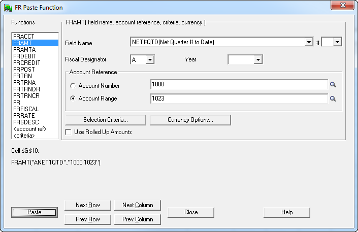
3. On the FR Paste Function screen, click the Next Column button.

   The cell reference (below the Functions list) changes to $G$10.

4. Specify a range of amounts to search.
   1. On the Functions list, click FRAMT.
   2. In the Field Name field, select NET#QTD(Net Quarter # to Date).
   3. On the Fiscal Designator list, select A (for Actual monetary figures).
   4. In the Account Reference group, select the Account Range option.
   5. Specify a range of accounts.
      1. In the first field in the Account Reference group, enter 1000.
      2. In the first field in the Account Reference group, enter 1023.
   6. If any accounts in the range are members of a rollup group and you want to view rolled-up amounts, select the Use Rolled Up Amounts option.

   The formula to be pasted into the spreadsheet appears below the Functions list. Show Me.

   

5. Click the Paste button to paste the formula into cell G10.
6. Click Close to close the FR Paste Function screen.

   In the spreadsheet, the net quarter to date amount appears in cell G10. (You may need to press F9 to recalculate.)

7. Save your work, and then close Excel.