Lesson 1: Using Formulas to Retrieve G/L Data
From Sage 300 ERP
Lesson 1: Using Formulas to Retrieve G/L Data
This lesson introduces Statement Designer functions and demonstrates how to construct basic statements that extract financial data from your general ledger.
-
Sign in to a sample company database. More...
Sage 300 ERP includes two sample databases you can use: SAMINC and SAMLTD. SAMINC has a single-currency general ledger with a US dollar functional currency. SAMLTD has a multicurrency general ledger with a Canadian dollar functional currency.
- Open Sage 300 ERP.
- Select SAMINC or SAMLTD.
- Enter ADMIN in the User ID and Password fields, and then click Open.
-
Open the Statement Designer. More...
-
Open General Ledger > Financial Reporter > Statement Designer.
- On the screen that appears, click Start to open a new Excel spreadsheet.
-
-
Turn off spreadsheet recalculation in Excel. More...
If spreadsheet recalculation is on, Excel will query the Sage 300 ERP database every time you enter a formula in the worksheet or navigate away from the FR View screen.
- Click File > Options.
- On the Formulas tab, in Calculation options, select Manual.
- Click OK.
Note: To update the worksheet with information from Sage 300 ERP, press the F9 key.
In this exercise, you will enter formulas manually in a spreadsheet to create a basic financial statement with account numbers, descriptions, and balances.
Tip: To avoid losing your work, click File > Save As, enter a file name, and save the file. Remember to save your work often as you work through the lessons in this tutorial.
- In cell F1, type =FR("Coname").
When you press Enter or select another cell, the company name appears in F1.
- In cell E3, type Account.
Note: If the content of a cell begins with a letter, the Statement Designer interprets that content as text. However, if you want to enter a number (such as 1999), you must type ="1999", so the program can interpret it correctly.
- In cell F3, type Description.
- In cell G3, type Balance.
- Select cells E3, F3, and G3.
- On the Home tab of the Excel ribbon, in the Font group, click the Borders
 button to add a bottom border.
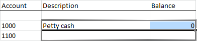
 - In cell E5, type ="1000".
Note: This is an account number, so you must enter it as a text string so the cell contents can be inserted in other formulas and interpreted correctly by Financial Reporter.
- In cell F5, type =FRACCT("ACCTDESC",E5).
The cell displays the account description for the account listed in cell E5.
- In cell G5, type =FRAMT("BALP",E5).
The cell displays the current balance for the account listed in cell E5.
- Press F9 to update the worksheet.
You have now created the beginning of a statement, with the headings for three columns and the information from one General Ledger account. Each formula you enter retrieves one piece of information from the General Ledger database. You can save the spreadsheet, and then view updated information the next time you open it.
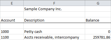
- In cell E6, type ="1100".
- Select cells F5 and G5, and then click and drag the bottom right corner of the selection border to copy the contents of F5 and G5 into F6 and G6.
The Statement Designer updates the copied formulas so they use account 1100 (cell E6) instead of account 1000 (cell E5).
- Press F9 to update the information in the copied formulas.
- Save your work.
The statement now appears as follows:
In this exercise, you will add column totals and format columns to prepare your financial statement for review and printing.
- Select cell G7.
- On the Home tab, in the Editing group, click the Autosum
 button.
Excel selects cells G5 and G6.
- Press Enter.
Cell G7 displays the sum of cells G5 and G6.
- Select cell G7 again.
-
On the Home tab of the Excel ribbon, in the Font group, click the arrow beside the Borders
button, and then click Top Border. - At the top of the spreadsheet, click column G to select all cells in that column.
- Right-click the column header for column G, and then click Format Cells.
- On the Category list, click Accounting.
- Accept the default selections for decimal places and currency symbol, or specify different settings if you prefer.
- Click OK.
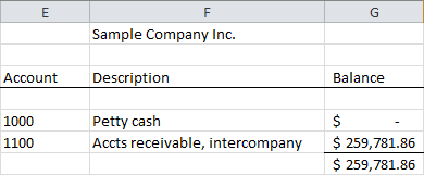
Amounts in column G are formatted as currency, using the decimal places and currency symbol you specified.
- Click and drag the edges of column headers to adjust the width of columns as needed to display information.
- Save your work.
The statement now displays two lines and the total balance for those lines, with balances formatted as currency:
- Continue to experiment with formatting commands by formatting and aligning column labels.
- Click File > Print to see a preview of the printed statement.
Next topic: Lesson 2: Using FR Paste to Insert Formulas