Chapter 3 - PhotoGrav Application
From PhotoGrav 3.0
 |
|
|
3.0 Introduction
Chapter Two described PhotoGrav’s operational
overview and how PhotoGrav uses these to provide a smooth flow of events
within a PhotoGrav
Session. This chapter, Chapter Three, provides a detailed description of each of
those primary functional blocks as well as describing a PhotoGrav Session
and the essentials of the PhotoGrav Application. The description with
appropriate graphics include: (1) PhotoGrav Sessions, (2) The Primary
Toolbar and its operations, (3) Viewing Panes and Panels, (4) Interactive Mode,
(5) Cloning—Comparison of Results, (6) Machine Selection, and (7) Automatic
Updates. It is especially recommended to become familiar with these primary
functional blocks located on the Primary Toolbar and the respective operations
since these are vital in producing a digital image for laser engraving.
3.1 PhotoGrav Sessions
One of PhotoGrav’s primary design concepts is the
notion of a “PhotoGrav Session” and its respective “Session File”
(*.pgs). A “Session File” is a file that is designed to save the current state
of ones work including all parameter settings, user preferences, machine and
material info, as well as the source image. By permitting the source
image to be saved with the session alleviates the need to remember where the
“original” image file is located. One can simply reopen the “Session File” and
perform any necessary modifications and/or adjustments without having to
relocate the original image. The machine information will be stored in the
“Session File” which is helpful, for example, if PhotoGrav is used with
multiple engravers. This permits one to save
machine/material “templates” such that the user can just open up the
session “template” pertaining to that particular machine/material and begin
using
PhotoGrav with the machine and material info already selected and
defined.
Whenever an image is opened, PhotoGrav will
automatically insert that image into either a new session OR an existing
active session. Either way there will always be only one image associated
with a PhotoGrav
Session.
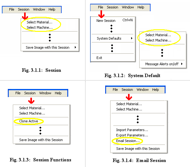
Due to the “Session File” format, however, one must keep in
mind that there are two modes of selecting a machine and/or material.
These two modes are selecting the “Session” machine/material (Figure 3.1.1) and
setting the “system” material/machine (Figure 3.1.2). The “Session” selection
stays with that particular session and the “System Default” selection sets the
default material/machine type so that any new session that is created will
default to the machine/material type that is selected in the “System Default”
settings.
Session files can be very useful when becoming proficient
with PhotoGrav in the following ways; when working with a difficult
image, if multiple engraving machines are used, when working with multiple
concurrent jobs, and in many other cases as well. PhotoGrav allows
multiple session files to be opened simultaneously and offers some functions
specifically related to Session files such as Cloning (Figure 3.1.3). For
further instruction on cloning refer to Section 3.5 on Cloning—Comparison of
Results .
PhotoGrav has the capability to email Session files
for easier review. For example PhotoGrav Session Files can be emailed to
PhotoGrav
Technical Support or to another office location for review simply by clicking on
the Session→Email Session… menu item (Fig 3.1.4).
From this point forward the majority of this section is in
the context of a “PhotoGrav Session” file (.pgs files).
3.2 Primary Toolbar
3.2.1 Overview
PhotoGrav is designed for simplicity, therefore, all
of the primary functions necessary to prepare an image for laser engraving are
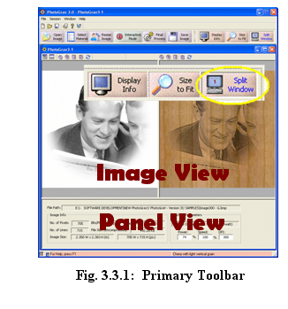
grouped together and displayed in the “Primary Toolbar” (Fig 3.2.1). The Primary
Toolbar provides quick access to the most commonly used functions.
Fig. 3.2.1: Primary Toolbar
The Primary Toolbar has 5 basic functions that perform the
minimum requirement operations to successfully laser engrave an image or
photograph. As noted in Section 2.1 of this manual these 5 minimal steps are as
follows:
- Open an Image (Input Image).
- Select the engraving material.
- Resize the image to the desired size.
- Process the image.
- Save the image to disk.
3.2.2 Open Image
![]()
The Open Image button simply displays a dialog window that
allows an image in any PhotoGrav supported file type (bmp, jpg, tif, png)
to be opened and inserted into either a new or existing session window. While
the open file dialog filters the listed items to only show PhotoGrav
supported image types. If the “All files (*.*)” option is selected any
PhotoGrav file type can be opened such as PhotoGrav Session Files
(pgs), PhotoGrav Parameter Files (prm, pgp), or PhotoGrav
Supported Image Files (bmp, jpg, tif, png).
The image that is initially opened is considered the
“Original Image”. The image can be either color or grayscale. PhotoGrav
then automatically converts the original image if necessary to a “Grayscale
Image”.
PhotoGrav considers the grayscale image because it is often much more
reliable to compare the grayscale image (rather than the color image) to the
engraved image.
3.2.3 Select Material
![]()
The “Select Material” button displays a dialog window listing
all the available materials sorted by the various categories (see Fig 3.2.2).
Remember that this material selection only changes the material for the “active”
session. Refer to Section 3.1, Fig 3.1.2 to see how to change the default
material setting. This list will be altered by the “Auto Update” feature (see
Section 3.7) as more materials become available for download. PhotoGrav
does not permit the user to modify this list due to the fact that many materials
individually and specifically tested and fine tuned for the best results. While
some material parameters are modifiable by the user there are a number of
parameters that are fixed during the design and testing phase of that material.
The material can also be chosen by double-clicking an item in the list or by
highlighting the material and clicking the “OK” button. The selected material
will then be displayed in the status bar at the bottom of the main application
window.
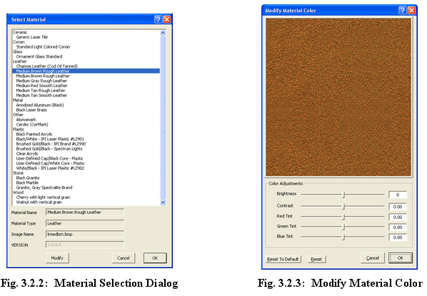
The Modify Material Color dialog window (Fig. 3.2.3)
can only be invoked from the Select Material dialog window and provides
the capability to the appearance of an engraving material. The capability to
modify the engraving material’s appearance enhances PhotoGrav’s
usefulness in two ways. The more important of the two ways is that it allows a
broad range of solid-color plastics to be effectively modeled by PhotoGrav.
This is achieved by providing two materials both of which have a User-Defined
Cap but one of which has a white core and the other has a black core. These
user-defined caps can be modified to have any solid color as will be described
below. The other way that the capability to modify the engraving material’s
appearance can be useful results from the fact that many engraving materials,
although similar to those provided by PhotoGrav, might differ somewhat in
color and brightness. The capability to alter their appearance might improve the
fidelity of the simulated engravings produced by PhotoGrav.
The material to be modified can be chosen by clicking a
material item in the list in Fig. 3.2.2 and then clicking the “Modify” button.
Pressing the “Modify” button causes the Modify Material dialog window to
appear.
The controls in the “Color Adjustments” frame are used to
modify the appearance of the engraving material. The “Brightness” and “Contrast”
controls affect the overall brightness and contrast of the material for all
colors equally. The “Brightness” modification can range from -100 to +100 and
the “Contrast” modification can range from -1.00 To + 1.00. The modification
values can be changed only by clicking the scrollbars, not by direct numerical
entries in the textboxes.
The “Red Tint”, “Green Tint”, and “Blue Tint” scrollbars
change the contrast of the respective colors. The tint modifications can range
from -1.00 to +1.00 and can be changed only by clicking the scrollbars, not by
direct numerical entries in the text boxes.
Modifications caused by the adjustments are immediately
visible in the material image view window. The “Reset” command button
resets all of the scroll bars to the “no adjustment” state since the last time
this material was modified. The “Reset to Default” button resets the
adjustments to the default setting of the material, in other words to the
settings of the material when originally shipped.
As an example try selecting the “User-Defined Cap/White Core”
material type under plastics. And click “Modify”. Then adjust the “Green Tint”
and “Blue Tint” slider bars so that both have a value of -1.00. Note that the
effect of these values is that the material image view window turns from white
to bright red. That red color could be further adjusted by changes in the
“Brightness”, “Contrast”, and “Red Tint” scroll bars. The net result is that one
can create almost any desired color for the cap of a solid-color plastic for
which the core color can be either white (in the example) or black.
3.2.4 Resize/Resample Image
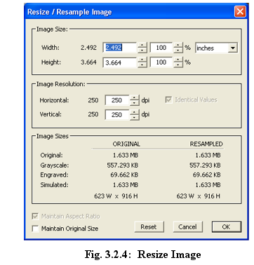
Resizing and/or Resampling the original input image (Fig 3.2.4) is almost always
a requirement because one rarely receives the image in the actual size needed
for engraving (this does vary some depending on the engravers policies).
PhotoGrav offers the ability to resize/resample an image to the desired
size without having to depend on other outside methods. PhotoGrav will
raise a notification if it detects a discrepancy between the selected machine
resolution (dpi) and the resolution (dpi) of the image. The image should be
resampled to the same resolution (or an integer multiple of) as the desired
engraving resolution (machine dpi setting). PhotoGrav uses the machine
settings extensively to prepare and simulate the image to give the user an idea,
estimate, or relative difference of what to expect when the actual engraving is
performed. Therefore, PhotoGrav does not adjust the “actual engraver”
setting, which is usually modified through the software driver that comes with
the engraver, but rather only adjusts the “machine setting” in PhotoGrav
which is then used to prepare the image for engraving.
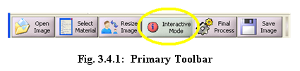
3.2.5 Final Process
![]()
The “Final Process” command button performs the actual
processing necessary to produce an image ready for the laser engraver. This
button should be pressed in every case prior to saving the image to disk. Once
the “Final Process” button is clicked PhotoGrav will process the image
using the current parameter settings. After the processing is complete
PhotoGrav will switch the image viewing pane to either the “Engraved” image
or the “Simulated” image determined by which image is selected in the viewing
pane toolbar (see Section 3.3, Fig 3.3.2). There will now be a total of three or
four images to use for comparison purposes in order to further fine tune the
results if needed.
3.2.6 Save Image
![]()
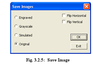
Now that the material has been selected and the image has
been opened, resized, and processed it is ready to be saved to disk for
engraving (Fig 3.2.5). To do this simply select the “Save Images” button on the
Primary Toolbar and save the appropriate images to disk in any of the
PhotoGrav
supported file formats. The only exception is the “Engraved” image which cannot
be saved as a jpeg due to the fact this format usually uses a lossy compression
type scheme which would create dire effects on the engraved image. One can elect
to save the images while flipping either horizontally, vertically or both. One
may find the “Flip Horizontal” check box to be turned on depending on the
material type selected due to the fact that some material types such as acrylic
engrave better on the back side, therefore requiring the image to be flipped or
mirrored. This can be altered, however, by modifying the parameters when in
Interactive Mode and then saving the session as a Template Session.
After the "Save Images" dialog is opened one
must select the “Exit” button to close out of this dialog screen. The reason for
this is that often it may be desirable to save more than just the “Engraved”
image so this goes into a continuous loop until all images are saved as needed.
3.2.7 Display Info
![]()
The remaining buttons on the Primary Toolbar have to do with
the way information is handled and viewed (see Fig 3.2.6). After pressing the
“Display Info” button the “PhotoGrav Session Report” window will be
displayed (Fig 1.6.1). This is a formatted report, that can be viewed or
printed, of the parameter, machine, and image settings for a particular session.
This report also includes thumbnail images of the original and simulated image
types. This provides an opportunity to print and file every job performed while
having quick access to all the data that was used for that job. One can also use
it to quickly view all the relevant settings for a session in a neatly organized
fashion. The PhotoGrav Session Report is also where an
estimate of the engraving time can be located and any comments that might be
helpful relating to the active session.
Fig. 3.2.6: Primary Toolbar
3.2.8 Size to Fit
The “Size to Fit” button zooms all the images to fit within
the viewing panes (see Section 3.3 for further information on Viewing Panes and
Panels).
3.2.9 Split Window
The “Split Window” button toggles between viewing the images
in a single or double viewing mode (see Section 3.3 for further information on
Viewing Panes and Panels).
3.3 Viewing Panes and Panels
 PhotoGrav provides a few options for displaying
information about the image, session, machine, parameter, etc. The session
window is divided up into 2 primary views. The first is the “Image” view. This
is where the images are displayed and image commands such as zoom in, zoom out,
pan, etc. are performed. Due to the numerous sizes and resolutions of existing
monitors
PhotoGrav offers the ability to view the images in either single or
“split window” mode. This allows for a larger viewing area where the images can
be cycled one at a time in single view mode or individually selectable by
pressing the corresponding toolbar button. On the other hand it also permits one
to compare side-by-side the resulting images in split screen mode (Fig 3.3.1).
PhotoGrav provides a few options for displaying
information about the image, session, machine, parameter, etc. The session
window is divided up into 2 primary views. The first is the “Image” view. This
is where the images are displayed and image commands such as zoom in, zoom out,
pan, etc. are performed. Due to the numerous sizes and resolutions of existing
monitors
PhotoGrav offers the ability to view the images in either single or
“split window” mode. This allows for a larger viewing area where the images can
be cycled one at a time in single view mode or individually selectable by
pressing the corresponding toolbar button. On the other hand it also permits one
to compare side-by-side the resulting images in split screen mode (Fig 3.3.1).
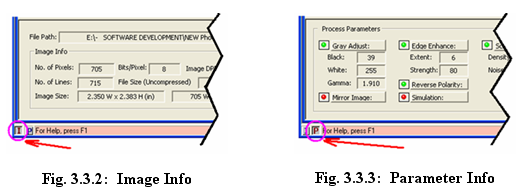
The second view that provides information is called the
“Panel” view. The “Panel” view is further divided into two subsequent views
named “Image Info” and “Parameter Info” (Fig 3.3.1). The “Image Info” panel (Fig
3.3.2) shows basic information about the image and the currently selected
machine. The next sub panel is the “Parameter Info” panel (Fig 3.3.3) which
displays a fixed summary of the current parameter settings. This “Parameter
Info” view changes to permit adjustments and modifications to the parameters
when in “Interactive Mode” which is discussed in Section 3.4.
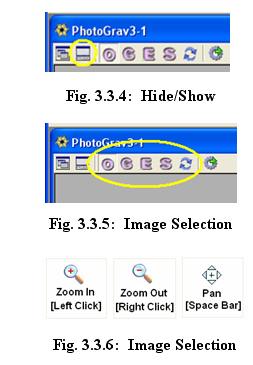
These panel views can be hidden to again provide for larger
viewing areas as needed by selecting the appropriate toolbar button from the
PhotoGrav Session Toolbar (Fig 3.3.4).
There are four images that one can select for viewing namely
Original input, Grayscale,
Engraved/binary, and the
Simulated images (Fig 3.3.5). If one has
“Split Screen” selected then these images can be selected independently per
image view. To open an image one can select the “Open Image” button on the
primary command bar. This button can be selected even if there is no session
window open in which case a new session window will be created and the
respective image inserted into that session. If, on the other hand, an existing
session is open then the selected image will be inserted over the existing image
if an image exists. In other words, if the user already has a session open then he
or she should create a “New” session prior to opening the image to prevent the
replacement of the existing session’s image.
By left or right clicking of the mouse button in either one
of the two Image View Windows one can incrementally zoom in or out respectively.
It is also possible to drag a zoom “box” or rectangle around the desired area
for closer inspection of the images. Another image command is the “pan” command.
This command centers the image at the point where the mouse button was clicked. Holding
down the [Space Bar] will activate this command (Fig 3.3.6).
3.4 Interactive Mode
The Interactive Mode Button toggles between two modes
of operation. When in "Interactive Mode" the Interactive Mode Button will
show a green “i” icon indicating that PhotoGrav is in
"Interactive Mode". Similarly when
PhotoGrav is NOT in “Interactive Mode” the button will display a
red “i”.
The “Interactive Mode” is designed for the primary purpose of
providing a quick and efficient preview of the final image, since with average
size images it would simply take too long to run through the entire PhotoGrav
processing pipeline every time a small change is made to a parameter. With this
in mind PhotoGrav distinguishes between “Preview” and “Final Process”.
The “Final Process” button (formerly called “Auto Process” in previous versions)
takes the raw image data along with the current material, parameter, and machine
settings and completely processes the image producing the binary or engraved
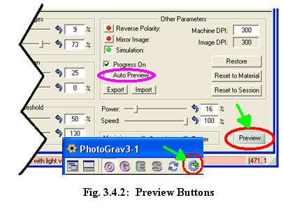
image ready to be saved and engraved. On the other hand the “Preview” buttons
(only available in “Interactive Mode” - Fig 3.4.2) process a scaled version of
the image (NOT THE ORIGINAL IMAGE) suitable for rapid viewing as one adjusts and
modifies the parameters in almost if not real time.
PhotoGrav does not restrict the image view display
size therefore providing a larger viewing area for a more accurate
representation of the resulting image. A larger viewing area does require more
processing speed in order to maintain real time performance. The real time
performance of interactively adjusting the parameter settings is a direct
correlation to the size of the image and the size of the display screens viewing
area. Since
PhotoGrav permits arbitrary screen sizes it is better prepared to adapt
to the increasing speeds of modern computers. Assuming 17” to 24” computer
monitors and current average to high end computers one can expect almost real
time performance when interacting with the parameters while in “Interactive
Mode”.
Due to the plethora of monitor and display types,
resolutions, and sizes that exist in the market place today PhotoGrav
offers a couple of options to facilitate the advanced user who relies on the
“Interactive Mode” in their production cycle. The first option is the “Auto
Preview” checkbox (Fig 3.4.2). This is provided to give the user the ability to
regenerate the preview image automatically after each parameter adjustment
without the user having to manually click on the “Preview” buttons. The user may
select to turn this on or off depending on the image size and/or display screen
size to increase performance. The second option is the “Progress Bar On”
checkbox (Fig 3.4.2). This checkbox offers the user the option of increasing
performance by turning this off. When the progress bar is turned off
PhotoGrav will process the “Preview” image slightly faster, however, with
larger images and depending on the speed of the users’ computer one may want to
turn this on. By turning this on it gives a “heads up” as to what PhotoGrav
is doing followed by an indication when the “Preview” image is ready for
display.
Once the image and parameters are determined either in
“Interactive Mode” or otherwise then the user can select the “Final Process”
button to process the image. Clicking on the “Final Process” button inherently
assumes that the user is now ready to prepare and process the image for
engraving and exporting. Once the final processing is complete one can
export/save the images or compare the images to other sessions (see Section 3.5
on Cloning—Comparison of Results later on).
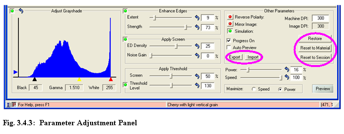
While working in “Interactive Mode” the user may want to
restore the parameters to a previous value. PhotoGrav provides parameter
restoration at 3 different levels (Fig 3.4.3). The first is “Restore” which
restores the parameter settings of the current session to the values it carried
along the last time that the image was processed using the “Final Process”
button. The second method of restoration is “Reset To System”. This resets the
parameters to the default settings of the base material selected for that
session. And finally the third level of restoring the parameters is “Reset To
Last Saved”. When one clicks this button it resets the parameters back to the
settings since the PhotoGrav Session was last saved.
It may be desirable to export or import (Fig 3.4.3) some
parameter settings while in Interactive Mode” and therefore PhotoGrav
offers these capabilities through the selection of the respective buttons.
PhotoGrav
allows the user to import parameter settings from version 2.xx (.prm files) or
version 3.xx and later (.pgp files), however, one can only export parameter
settings in version 3.xx and above “pgp” format. The parameters can also
be exported or imported via the menu bar at the top of the PhotoGrav
Application Window.
The remaining comments in this section describe the various
parameter settings and the respective controls. PhotoGrav has five major
processing functions whereby it transforms the original input image into the
Engraved and Simulated images. All processing function can be toggled on or off
by clicking on the small green or red lights beside each processing function
turning the functions on or off respectively. Furthermore, all processing
functions can be quickly reset by pressing the small blue “Reset” arrow beside
each control function.
3.4.1 Adjust Grayshade
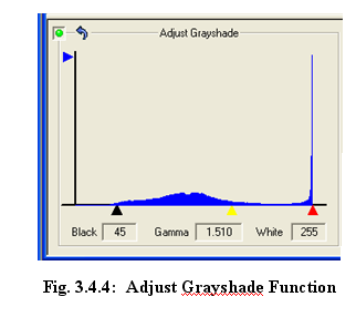
Figure 3.4.4 displays a histogram, or distribution, of the
gray shades in the Original (input) image. The horizontal axis ranges from zero
(black) on the left to 255 (white) on the right. The height of the distribution
indicates the relative number of image elements (pixels) that have the gray
shade indicated by the corresponding point on the horizontal axis. (If a
distribution is very “peaked” at certain gray shades, then the peaks are
truncated and other heights scaled to prevent the peaks from totally dominating
the distribution). As an example, for the distribution displayed in Fig. 3.4.4,
there are many more values of “white” in the image compared to any other gray
shade producing a large spike at the very far right of the histogram. The rest
of the histogram looks to have a higher concentration of values near the middle
of the gray shaded spectrum.
The left (black) and right (red) triangles below the
horizontal axis specify the black and white clipping values, respectively, for
the “Adjust Grayshade” function, i.e., all grayshades to the left of the left
triangle are set to black (zero) and all grayshades to the right of the right
triangle are set to white (255) and the grayshades between are linearly scaled.
The “Black” and “White” labels to the left of the distribution specify
quantitatively the black and white clipping values (45 and 255, respectively,
for the distribution in Fig. 3.4.4). The clipping values can be changed by
“clicking and dragging” the triangles. As a result, the “Black” and/or “White”
quantitative values will change and the effect will show up as a change in the
Processed and simulated Image. The clipping values can also, of course, be reset
by clicking the small blue “Reset” arrow. (Note: All the engraving
materials delivered with PhotoGrav calculate the “1%” clipping values for
the grayshade distribution).
The middle (yellow) triangle below the horizontal axis is the
“gamma” for the gray shade transfer function. Changing the gamma value, by
clicking and dragging the triangle, has the effect of simultaneously changing
the brightness and contrast of the image. Moving the triangle to the right will
generally make the Processed Image brighter and moving it to the left will
generally make it darker.
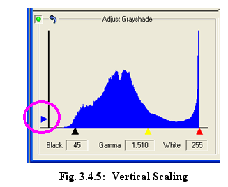
The blue triangle (Fig 3.4.5) that slides in the vertical
direction located on the left side of the histogram provides a scaling function
so that a few values do not dominate the graph. Note that in Figure 3.4.5 the
histogram shows a much more evenly distributed display thus far more readable.
Both Figure 3.4.4 and Figure 3.4.5 are the exact same histogram but note how the
two blue vertical triangles have different locations. By adjusting this vertical
scaling triangle a much more readable view of the image distribution is
achieved.
3.4.2 Enhance Edges
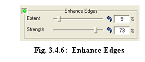
The “Enhance Edges” function provides the capability
to both “smooth” the image and to enhance the image’s edges. As with the “Adjust
Grayshade” function, if the green “On” button is checked, then the
function affects the image data; otherwise, if unchecked (red), there is NO
effect regardless of the parameter settings.
The “Extent” parameter pictured in Fig. 3.4.6 can be
modified by entering a value directly in the appropriate textbox (contains “9”
in Fig. 3.4.6) or by clicking the associated horizontal scrollbar. The "Extent"
parameter specifies the relative size of the area around each pixel which is
then smoothed. Small values indicate relatively little smoothing whereas large
values specify relatively large smoothing.
The “Strength” parameter specifies the degree to which
edges are enhanced or emphasized . The “Strength” parameter is controlled
in a manner similar to the “Extent” parameter except that its values
range from -100% to +100% rather than 0% to 100%. Almost all of the useful
settings for the “Strength” parameter are positive but interesting
effects can sometimes be achieved with negative settings.
Although PhotoGrav automatically sets parameter values
appropriate to each engraving material, it is a good idea for you to experiment
with the “Extent” and “Strength” parameter settings to get a feel
for their effect which at times can be rather dramatic. An interesting way to do
this is to have the “Simulation” ON and to turn the “Enhance Edges”
function alternately ON and OFF to observe the effect.
3.4.3 Apply Screen
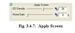
The “Apply Screen” function (Fig. 3.4.7) provides the
capability to “screen” the image in preparation for thresholding which follows
this function.
The “Apply Screen” function actually performs a
Diffusion Dithering. Diffusion Dithering is a technique to convert a grayshade
image to a binary image (black & white only, no shades of gray) wherein the
shades of gray in the original image are represented in the processed binary
image by differing densities of black and/or white dots. Diffusion Dithering
accomplishes this by converting each gray shade in the original image to either
a black or white value depending on its value relative to a predetermined
“threshold” value. The error in making this assignment is then “diffused” to
neighboring pixels which eventually are also thresholded (and then error
diffused) and so forth and so on throughout the entire image.
The Diffusion Dithering within PhotoGrav has been
designed and optimized specifically for laser engraving and is controlled by the
two parameters indicated in Fig. 3.4.7: (1) ED Density and (2) Noise
Gain. (The ED stands for Error Diffusion). The “ED Density” parameter
can be used to darken lighter areas of the processed image without substantially
affecting areas that are already dark and, vice versa, can be used to lighten
darker areas of the image without substantially affecting areas that are already
light. The “Noise Gain” parameter can be used to add noise to the image
to reduce “contouring”, "repetitive pattern", or “jpeg artifacts” effects that
often occur when grayshade images are converted to binary images.
Both parameter values can be modified by clicking the scroll
bars or by entering numeric values in the white text boxes directly above each
scroll bar. Relative values for the “ED Density” parameter range from
-100 (darken) to +100 (lighten). Relative values for the “Noise Gain”
parameter range from 0% (no noise) to 100% (maximum noise).
3.4.4 Apply Threshold
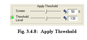
The “Apply Threshold” function (Fig 3.4.8) linearly
combines the last two control functions (Enhance and Screen), pixel by pixel and
with variable weights, before thresholding the result to create an
“Engraver-ready” binary image.
There are two parameters associated with the “Threshold”
function: (1) the “Screen %” and (2) the “Output Threshold Level”.
The first parameter, the “Screen %”, specifies how the two inputs to the
function are combined by specifying the weighting factor assigned to the input
from the “Screen” function. The weighting factor assigned to the image coming
from the “Enhance” function is then equal to (100 - Screen %) . A value of zero
for this parameter specifies that the resulting data, before thresholding, is
totally from the “Enhance” function. A value of “100” for this parameter
specifies that the data, before thresholding, is totally from the “Screen”
function. A value of “50” for this parameter specifies that the two inputs are
equally weighted and then combined. The “combine” portion of the “Threshold”
function is always ON, i.e., the two inputs are ALWAYS combined, before
thresholding, using the weighting factors specified by the “Screen %”
factor.
The second parameter, the “Threshold Level”, specifies
a threshold value which ranges from zero to 255. The threshold value is applied
to the combined output of the “Enhance” and “Screen” functions, weighted as
described above. If a combined value is less than the threshold value, then it
is assigned a zero (black). If a combined value is greater than the threshold
value, then it is assigned a one (white). The “threshold” portion of this
function, unlike the “combine” portion, can be turned ON or OFF by checking, or
not checking, the green/red checkbox located to the left of the label “Threshold
Level”. If the thresholding is OFF, then the simulation function, described in
the next section, cannot be turned ON and an engraver-ready (binary) image is
not produced.
Either parameter for this function can be modified by
clicking the horizontal scroll bars or by entering a numeric value in the white
text boxes immediately below the scroll bars.
3.4.5 Speed and Power
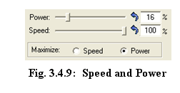
The vertical scroll bars labeled “Power” and “Speed”
(Fig 3.4.9) specify the percentage of maximum power and the percentage of the
maximum speed for the laser engraver currently being modeled (You can change the
laser engraver being modeled as well as the specifications for any laser
engraver by selecting a different machine see Section 3.6). The “Power”
and “Speed” controls should be very similar to the controls which
actually exist on your laser engraver and should behave in the same fashion.
The “Maximize Power” and “Maximize Speed” (Fig
3.4.9) checkboxes determine whether the Power setting or Speed
setting for your machine is maximized when it is necessary to modify these
settings. The necessity for modifying these settings occurs since PhotoGrav’s
engraving materials were calibrated using a specific machine; therefore the
power, speed, resolution, etc. of your machine may not match those of
the “calibration” machine. PhotoGrav
strives to deliver the appropriate quantity of energy to each laser spot, based
on the settings for your machine, and in so doing has a choice of what values to
use for the Power and Speed settings (generally a large number of
settings will all satisfy the energy requirement). If you are interested in
engraving as fast as possible, then the “Maximize Speed” box should be
checked. If you are more comfortable with a higher Power setting, then
the “Maximize Power” box should be checked. These two boxes cannot both
be checked or unchecked at the same time so the boxes also act as toggles, i.e.,
if you check the “Maximize Power” box, then the “Maximize Speed”
box will automatically become unchecked and vice versa. (Note: The effect of
these checkboxes may at times appear confusing and it may at first appear to you
that they are not working properly. It is important to remember that “Maximize”
is used for both boxes to mean the maximum value for that parameter that will
still result in the proper energy being delivered to the laser spot
and that maximum value may not be 100%. For example, if the “Maximize Speed”
box is checked, then it would be possible for the Power and Speed
settings to be, e.g., 100% and 65%, respectively, which might at first seem
incorrect since “Speed” was to have been maximized. However, in the
example given, if the Speed is more than 65%, then inadequate energy will
be delivered to the laser spot since the Power setting cannot be more
than 100% (Speeding the engraver up delivers less energy to each spot). So, in
this case, 65% is indeed the “maximum” value for the Speed setting
subject to the constraint that the proper quantity of energy is delivered to the
laser spot).
3.4.6 Other Parameters
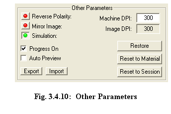
The remaining parameter settings and various other functions
are located under the “Other Parameters” group box.
The text box labeled “Machine DPI”, containing the
value 300 in Fig 3.4.10, specifies the Engraver resolution, NOT the image
resolution, in dots per inch. The value in this textbox is initially taken from
the dpi value selected from the “Machine Preferences” dialog box. It
should be noted that when changing the “Machine DPI” will only cause the DPI
setting to become the Engraver resolution for the current session. The textbox
labeled “Image DPI” is for reference only and thus cannot be altered by
the user.
The “Reverse Polarity” checkbox provides the
capability to set the polarity of the Engraved and Simulation images. Positive
polarity materials are those for which the laser, when on, causes the engraving
material to become darker, e.g., most woods. Negative polarity materials are
those for which the laser, when on, causes the engraving material to become
lighter, e.g., black laser brass and acrylics. The “Mirror Image”
checkbox provides the capability to “mirror-the-image” (flip left to right) the
Engraved and Simulation images. This feature is useful for materials like
acrylic which are engraved on the “back” of the engraving material but viewed
from the front. For various reasons the processed image is not shown “mirrored”
in the Image Viewing Windows, but rather the Engraved and Simulated images are
flipped (by user selection) only when written to disk.
A few other options are also available such as turning the
Simulation on or off as well as exporting or importing parameters either from
the current or previous versions of PhotoGrav. Refer to the beginning of
this Section (3.4) for further information on most of these settings and
functions.
See Section 2.2 for a more complete discussion of the underlying
rationale for the simulation capability and how it can be an extraordinarily
useful tool.
3.5 Cloning—Comparison of Results
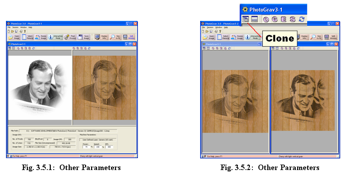
The comparison of images whether simulated or otherwise can
be an efficient time saving procedure when it comes to preparing the image for
engraving. PhotoGrav offers two different methods by which one can
compare the processed image. The first is to compare the various images solely
within a particular session (Fig 3.5.1) and second is to compare the results of
two sessions with each other (Fig 3.5.2).
Learning how to use the “Cloning—Image Comparison” features
along with the simulation of results should again increase productivity. While
the simulation is attempting to get as close as possible to the final results
there are many variables that affect the results of the actual vs. the simulated
images. Therefore, the simulation can be thought of as a relative comparison of
the simulated images rather than an absolute final result. This essentially
means that once one learns how a particular “simulated” image compares to the
actual engraved image for a specific material and machine type; then a
“relative” difference or pattern should emerge giving the user a sense of how to
adjust the parameters to improve the actual engraving. This simulation feature
was significantly relied on during the design of PhotoGrav to improve
performance and efficiency.
PhotoGrav has a “Clone” function (Fig 3.5.2) to
further assist in comparing processed results. This “Clone” feature
assumes that the user wants to spin off or clone another session based on the
current active session. This provides an exact duplicate of the current selected
session or active session. This provides an efficient method to quickly process
another session and compare the two (if desired) without having to go through
the whole process of reopening the same image in another session. For example,
it can be helpful to compare one simulated or engraved image (session X), where
the parameters have been adjusted, with a second image (session Y) where the
parameters have NOT been modified (i.e. default material settings).
3.6 Machine Properties
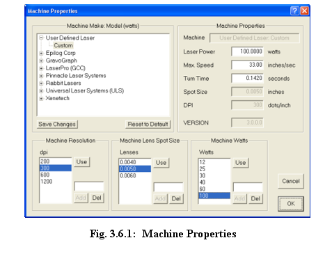
The “Machine Properties” dialog window (Fig. 3.6.1)
can only be invoked from the main application menu bar and is used to select and
modify the laser engraver and associated parameters which PhotoGrav is
currently modeling. The “Machine Make” frame provides the capability for you to
select your laser engraver manufacturer and model type. The “Machine
Properties”, “Machine Resolution”, “Machine Lens Spot Size”,
and “Machine Watts” frames provide the capability for you to modify, add
to, or specify completely, the parameters that essentially define the laser
engraver model.
The list at the top of the “Machine Model” frame displays the
laser engraver machines currently modeled by PhotoGrav including a “User
Defined Laser” machine for which you can completely specify the engraver
parameters from scratch. Each machine manufacturer in the list also provides a
“Generic” laser model type in the case where the specific model type is not known
but the manufacturer is known. In the case of the “Generic” model type all the
machine properties can be defined just as in the “User Defined Laser” case.
Selecting a machine from the list will enter the machine’s
name into the text box directly to the right of the list along with the machine
model type. It will also change all the settings to reflect which machine type
is selected.
Clicking the “Reset to Default” button will restore a
machine’s parameters, to the values they had when PhotoGrav was first
installed, for whatever machine is currently selected. Any machine’s parameters
can be modified using the controls in the “Machine Properties” dialog
window and, once the “OK” button is pressed, the modified parameters become the
current parameters for the machine and are stored to disk as such when the
current PhotoGrav session terminates).
The first two textboxes at the top of the “Machine
Properties” frame specify the maximum power (in watts) and the maximum speed
(in inches/second) for the current laser engraver. These two values obviously
have a big influence on how PhotoGrav produces the Simulated Image. The
third textbox from the top specifies the time, in seconds, for the laser to slow
down, stop, and reverse direction for each scan line. This parameter is used
only for calculating estimates of the engraving time, which are displayed in the
PhotoGrav Session Report (see Section 3.2.7). A procedure for calculating
this parameter for your particular machine is presented in Appendix 3:
Calculational Procedure for “Turn Time”.
 The list displayed in the “Machine Lens Spot Size” frame contains a list of the
effective laser spot sizes (diameters in inches) for the lenses available to the
simulated Laser Engraver. These are the values that are available to
PhotoGrav
for creating the Simulated Image. A single click of an item in the list only
locally selects the item. When an item in the property listbox is selected two
functions can be performed, namely “Del” or “Use”. The “Del” button deletes the
item from the list while the “Use” button places that value into the associated
text under the “Machine Properties” frame. Double clicking on a list item will
behave just as if the “Use” button was pressed. Also, values in the list textbox
can be Added to the list by clicking the “Add” button.
The list displayed in the “Machine Lens Spot Size” frame contains a list of the
effective laser spot sizes (diameters in inches) for the lenses available to the
simulated Laser Engraver. These are the values that are available to
PhotoGrav
for creating the Simulated Image. A single click of an item in the list only
locally selects the item. When an item in the property listbox is selected two
functions can be performed, namely “Del” or “Use”. The “Del” button deletes the
item from the list while the “Use” button places that value into the associated
text under the “Machine Properties” frame. Double clicking on a list item will
behave just as if the “Use” button was pressed. Also, values in the list textbox
can be Added to the list by clicking the “Add” button.
PhotoGrav adjusts itself appropriately so that the simulated
engraving is as realistic as possible. The lens that is installed on the laser
engraver is the lens that should be specified in this textbox. Generally, for
photographs, the spot size corresponding to the highest-resolution is the best
lens to use, if that lens is available for your machine.
The second list is the “Machine Resolution” frame which
contains a list of the resolutions (dots per inch) available to the simulated
Laser Engraver. The controls in this frame behave identically to the controls in
the “Machine Lens Spot Size” frame as described in the paragraph above.
Similarly, the “Machine Watts” frame behaves just as the other two similar
frames.
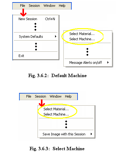
It is important to remember that there are two locations where
the “Machine Properties” can be selected. The first one is located under the
File→System Defaults→Select Machine… menu item (Fig 3.6.2). When this option
is selected ONLY THE DEFAULT MACHINE TYPE IS CHOSEN which means
that any new session that is created will use this machine type. The
second method of opening the “Machine Properties” dialog window is located in
the Session→Select Machine… menu item (Fig 3.6.3). When this method is
used ONLY THE ACTIVE SESSION MACHINE PROPERTIES ARE MODIFIED.
3.7 Automatic Updates
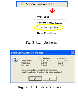
Another feature that can be very useful in PhotoGrav
is the ability for additional materials and machine types (when available) to be
added automatically via an internet connection on any computer that has
PhotoGrav
installed (Fig 3.7.1). This does not prevent one from still saving/exporting and
loading/importing parameter files and PhotoGrav Sessions (pgp
files) for both current and previous versions of PhotoGrav and
custom configuring the machine settings as required.
The available method to check for updates is through the Help
menu item as shown in Figure 3.7.1. There are three main items that
PhotoGrav
checks for when performing a “Check for Update” function. The first and second
are to check for any new Materials and Machines. The third is to check for any
updates to the application. If any one of these three checks indicates a need to
update then a message listing the current vs. latest versions available (Fig
3.7.2) appears. The updates can then be selected to “Yes” go ahead and download
or “No” just leave it as it is.