9. Performing a Pole-Zero Analysis

You can use the LabVIEW System Identification Assistant to compute the poles and zeros of the transfer function for one input-output pair of a model. The Pole-Zero Analysis step computes the pole-zero plot for a model.

Complete the following steps to perform a pole-zero analysis of the ARX model.

1. In the Project View, right-click the Parametric Estimation step and select Insert After»System Identification»Model Analysis»Pole-Zero Analysis from the shortcut menu to add a Pole-Zero Analysis step after the Parametric Estimation step.
2. On the Input Model tab in the Configuration View, verify that ARX Model is selected in the Model pull-down menu. ARX Model is the only model output from previous steps and therefore appears by default in this menu.
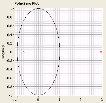
3. The Pole-Zero Plot displays the poles and zeros of the ARX model. Notice that all the poles of the plot are inside the unit circle, which indicates that the system is stable. A stable system reaches a steady-state value.
   
   Also notice that the poles are on the real axis, which illustrates the monotonic nature of the signal. Poles with imaginary components indicate an oscillating signal.
4. You can set the minimum and maximum values of the x- and y-scales of the plot to resize the plot. Click the maximum value on the x-axis and change the value to 3. Notice the zero on the Pole-Zero Plot, as shown in the following figure.
   
   
5. Select File»Save Project to save the project.