Designing a Floating-Point Filter Part 2: Analyzing a Digital Filter (Digital Filter Design Toolkit)
In Part 1 of this tutorial, you learned how to create and specify a floating-point filter design by using the Classical Filter Design Express VI. In Part 2 of this tutorial, you analyze the characteristics of the filter by evaluating the magnitude response of the filter.
Note If you did not complete Part 1 of this tutorial, refer to labview\examples\Digital Filter Design\Getting Started\Tutorials\Designing a Floating-Point Filter\Designing a Floating-Point Filter Part 1.vi for a completed version of the digital filter from that part.
Complete the following steps to analyze a filter design by using the Filter Analysis Express VI.
Place the Filter Analysis Express VI on the block diagram.
Place
Find
The Configure Filter Analysis dialog box appears with Sample Data labels on the graphs. These labels remain on the graph until you run the VI.
Leave the default settings and click the OK button to close the dialog box and return to the block diagram.
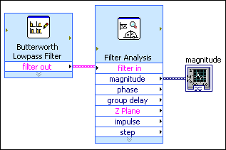
Wire the filter out output of the Classical Filter Design Express VI to the filter in input of the Filter Analysis Express VI.
Click the Run button to run the VI.
Double-click the Filter Analysis Express VI to open the configuration dialog box and view the graphical analysis of the filter.
Click the OK button to close the dialog box and return to the block diagram.
Right-click the magnitude output of the Filter Analysis Express VI and select Create»Graph Indicator from the shortcut menu.
A new indicator appears to the right of the Filter Analysis Express VI. This indicator represents a waveform graph in the front panel window. This graph displays data from the magnitude output of the Filter Analysis Express VI.
The block diagram now resembles the following figure.
Double-click the magnitude indicator to display the front panel window of the VI and see the graph.
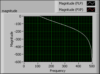
Click the Run button to run the VI. The following figure displays the magnitude graph of the filter design.
Note Graph indicators you create from the Filter Analysis Express VI automatically show two lines on the plot legend to facilitate comparison between floating-point and fixed-point filters. In this tutorial, only the graph for the floating-point filter appears.
In the previous figure, notice the filter passes frequencies below 100 Hz with a 0.1 dB passband ripple and attenuates frequencies above 200 Hz with a minimum attenuation of 60 dB. This behavior is in accordance with the filter specifications you specified in Part 1.
(Optional) Create graph indicators for other outputs of the Filter Analysis Express VI, such as the phase delay, group delay, Z Plane, impulse, and step outputs. Then, display the front panel window and run the VI again.
Select File»Save to save the VI.
Designing a filter is a trial-and-error process. If the filter does not meet the filtering requirements, you can modify the filter specifications and analyze the filter again. After you design an appropriate filter, you can use the filter to process an input signal in Part 3 of this tutorial.
Note Refer to labview\examples\Digital Filter Design\Getting Started\Tutorials\Designing a Floating-Point Filter\Designing a Floating-Point Filter Part 2.vi for a completed version of the digital filter from this part of the tutorial.

 Place
Place