Understanding Dynamic System Models (Control Design and Simulation Module)
A dynamic system model is a mathematical representation of the dynamics between the inputs and outputs of a dynamic system. You generally represent dynamic system models with differential or difference equations. The following figure shows a sample dynamic system.
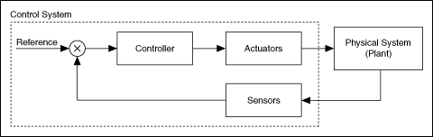
The dynamic system in the previous figure represents a closed-loop system, also known as a feedback system. In closed-loop systems, the controller monitors the output of the plant and adjusts the actuators to achieve a specified response.
You can use physical laws or experimental data to develop a dynamic system model. The following sections describe features of both the physical modeling and the empirical modeling techniques.
Physical Models
The laws of physics define the physical model of a system. The following sections describe various classifications and features of physical models.
Lumped versus Distributed Parameter Models
If you can use an ordinary differential equation to describe a physical system, the resulting model is a lumped parameter model. If you can use a partial differential equation to describe a system, the resulting model is a distributed parameter model.
Linear versus Nonlinear Models
Dynamic system models are either linear or nonlinear. A linear model obeys the principle of superposition and homogeneity. The following equations are true for linear models.
y1 = f(u1)
y2 = f(u2)
f(u1 + u2) = f(u1) + f(u2) = y1 + y2
f(au1) = af(u1) = ay1
where u1 and u2 are the system inputs, y1 and y2 are the system outputs, and a is a constant.
Conversely, nonlinear models do not obey the principles of superposition or homogeneity. Nonlinear effects in real-world systems include saturation, dead-zone, friction, backlash, and quantization effects; relays; switches; and rate limiters. Many real-world systems are nonlinear, though you can linearize nonlinear models to simplify a design or analysis procedure.
Time-Variant versus Time-Invariant Models
Dynamic system models are either time-variant or time-invariant. The parameters of a time-variant model change with time. For example, you can use a time-variant model to describe the mass of an automobile. As fuel burns, the mass of the vehicle changes with time.
Conversely, the parameters of a time-invariant model do not change with time. For an example of a time-invariant model, consider a simple robot. Generally, the dynamic characteristics of robots do not change over short periods of time.
Continuous versus Discrete Models
Dynamic system models are either continuous or discrete. Both continuous and discrete system models can be linear or nonlinear and time-invariant or time-variant. Continuous models describe how the behavior of a system varies continuously with time, which means you can obtain the properties of a system at any certain moment from the continuous model. Discrete models describe the behavior of a system at separate time instants, which means you cannot obtain the behavior of the system between any two sampling points.
Continuous system models are analog. You derive continuous models of a physical system from differential equations of the system. The coefficients of continuous models have clear physical meanings. For example, you can derive the continuous transfer function of a resistor-capacitor (RC) circuit if you know the details of the circuit. The coefficients of the continuous transfer function are the functions of R and C in the circuit. You use continuous models if you need to match the coefficients of a model to some physical components in the system.
Discrete system models are digital. You derive discrete models of a physical system from difference equations or by converting continuous models to discrete models. In computer-based applications, signals and operations are digital. Therefore, you can use discrete models to implement a digital controller or to simulate the behavior of a physical system at discrete instants. You also can use discrete models in the accurate model-based design of a discrete controller for a plant.
Empirical Models
Empirical models use data gathered from experiments to define the mathematical model of a system. To some degree, physical models are empirical because you experimentally determine certain constants used to develop the model. A variety of empirical modeling methods exist. One method of empirical modeling uses tables of experimental data that represent the system you want to model. Another method for developing models uses system identification methods. System identification methods use measured data to create differential or difference equation representations that model the data.
 |
Note You can use the LabVIEW System Identification Toolkit to construct models by using system identification methods. |
Linear Model Forms
You can use the Control Design and Simulation Module to represent continuous and discrete linear models in the following three forms:
- Transfer Function—These models use polynomial functions to define the relationship between the inputs and outputs of a dynamic system. You analyze transfer function models in the frequency domain.
- Zero-Pole-Gain—These models are transfer function models that you rewrite to show the gain and the locations of the zeros and poles of the dynamic system. You analyze zero-pole-gain models in the frequency domain.
- State-Space—These models represent the dynamic system in terms of physical states. Continuous state-space models use first-order differential equations to describe the dynamic system, whereas discrete state-space models use first-order difference equations. You analyze state-space models in the time domain.
SISO vs. MIMO Models
When you configure a continuous or discrete transfer function, zero-pole-gain, or state-space function, you can use the configuration dialog box to specify whether a function is single-input single-output (SISO) or multiple-input multiple-output (MIMO). SISO models have only one input and one output, whereas MIMO models have two or more inputs or outputs. You make this choice by selecting the appropriate option from the Polymorphic instance pull-down menu.