PxVehicleWheelData

mRadius:

This is the distance in metres between the centre of the wheel and the outside rim of the tire. It is important that the value of the radius closely matches the radius of the render mesh of the wheel. Any mismatch will result in the wheels either hovering above the ground or intersecting the ground. Ideally, this parameter will be exported from the 3D modeller.

mWidth:

This is the full width of the wheel in metres. This parameter has no bearing on the handling but is a very useful parameter to have when trying to render debug data relating to the wheel/tire/suspension. Without this parameter it would be difficult to compute coordinates for render points and lines that ensure their visibility. Ideally, this parameter will be exported from the 3D modeller.

mMass:

This is the combined mass of the wheel and the tire in kg. Typically, a wheel has mass between 20Kg and 80Kg but can be lower and higher depending on the vehicle.

mMOI:

This is the component of the wheel's moment of inertia about the rolling axis. Larger values make it harder for the wheel to rotate about this axis, while easier values make it easier for the wheel to rotate about the rolling axis. Another way of expressing this is that a high MOI will result in less wheel spin when stamping on the accelerator because it is harder to make the wheel spin. Conversely, lower values of MOI will result in more wheel spin when stamping on the accelerator.

If the wheel is approximately cylindrical then a simple formula can be used to compute MOI:

MOI = 0.5 * Mass * Radius * Radius

There is no reason, however, to rely on equations to compute this value. A good strategy for tuning this number might to be start with the equation above and then make small tweaks to the value until the handling is as desired.

mDampingRate:

This value describes how quickly a freely spinning wheel will come to rest. The damping rate describes the rate at which a freely spinning wheel loses rotational speed. Here, a freely spinning wheel is one that experiences no forces except for the damping forces arising from the wheel's internal bearings. Higher damping rates result in the wheel coming to rest in shorter times, while lower damping rates result in the wheel maintaining speed for longer. Values in range (0.25, 2) seem like sensible values. Experimentation is always a good idea, even outside this range. Always exercise some caution with very small damping rates. In particular, a damping rate of exactly 0 should be avoided.

mMaxBrakeTorque:

This is the value of the torque applied to the wheel when the brakes are maximally applied. Higher torques will lock the wheel quicker when braking, while lower torques will take longer to lock the wheel. This value is strongly related to the wheel MOI because the MOI determines how quickly the wheel will react to applied torques.

A value of around 1500 is a good starting point for a vanilla wheel but a google search will reveal typical braking torques. One difficulty is that these are often expressed by manufacturers as braking horsepower or in "pounds inches". The values required here are in "Newton metres".

mMaxHandBrakeTorque:

This is the same as the max brake torque except for the handbrake rather than the brake. Typically, for a 4-wheeled car, the handbrake is stronger than the brake and is only applied to the rear wheels. A value of 4000 for the rear wheels is a good starting point, while a value of 0 is necessary for the front wheels to make sure they do not react to the handbrake.

mMaxSteer:

This is the value of the steer angle of the wheel (in radians) when the steering wheel is at full lock. Typically, for a 4-wheeled car, only the front wheels respond to steering. In this case, a value of 0 is required for the rear wheels. More exotic cars, however, might wish front and rear wheels to respond to steering. A value in radians equivalent to somewhere between 30 degrees and 90 degrees seems like a good starting point but it really depends on the vehicle being simulated. Larger values of max steer will result in tighter turns, while smaller values will result in wider turns. Be aware, though, that large steer angles at large speeds are likely to result in the car losing traction and spinning out of control, just as would happen with a real car. A good way to avoid this is to filter the steer angles passed to the car at run-time to generate smaller steer angles at larger speeds. This strategy will simulate the difficulty of achieving large steer angles at high speeds (at high speeds the wheels resist the turning forces applied by the steering wheel).

mToeAngle:

This is the angle of the wheel (in radians) that occurs with no steer applied. The toe angle can be used to help the car straighten up after coming out of a turn. This is a good number to experiment with but is best left at 0 unless detailed tweaks are required.

To help the car straighten up apply a small negative angle to one of the front wheels and a small positive angle to the other front wheel. By choosing which wheel takes the positive angles, and which the negative, it is straightforward to make the wheels either "toe'in" or "toe'out". A "toe-in" configuration, the front wheels pointing slightly towards each other, should help the car straighten up after a turn but at the expense of making it a little harder to turn in the first place. A "toe-out" configuration can have the opposite effect. Toe angles greater than a few degrees are best avoided.

PxVehicleWheelsSimData

void setSuspTravelDirection(const PxU32 id, const PxVec3& dir):

This is the direction of the suspension in the downward direction in the rest configuration of the vehicle. A vector that points straight downwards is a good starting point.

void setSuspForceAppPointOffset(const PxU32 id, const PxVec3& offset):

This is the application point of the suspension force, expressed as an offset vector from the center of mass of the vehicle's rigid body. Another way of expressing this is to start at the center of mass of the rigid body, then move along the offset vector. The point at the end off the offset vector is the point at which suspension forces will be applied.

In a real vehicle the suspension forces are mediated through the suspension strut. These are often incredibly complex mechanical systems that are computationally expensive to simulate. As a consequence, instead of modelling the details of the suspension strut, it makes sense to assume that the suspension strut has an effective point at which it applies the force to the rigid body. Choosing that point, however, needs careful consideration. At the same time, it opens up all sorts of tweaking possibilities, freed from the constraints of the real world.

Deciding on the suspension force application point requires some thought. The suspension is very close to the wheel so the wheel center is a good starting point. Consider a line through the wheel center and along the suspension travel direction. Somewhere along this line seems like an even better idea for the application point, albeit not completely scientific. For a standard 4-wheeled car it makes sense that the application point is somewhere above the wheel center but below the centre of mass of the rigid body. It is probably above the wheel centre because the suspension is mostly above this point. It can be assumed that it is somewhere below the rigid body centre of mass because otherwise vehicles would lean out of the turn rather than in to the turn. This narrows down the application point to really quite a small section of a known line.

When editing the suspension force application point it is important to bear in mind that lowering the app point too far will result in cars leaning more into the turn. This can have a negative effect on handling because the inner wheel can take so much load that the response saturates, while the outer wheel ends up with reduced load and reduced turning force. The result is poor cornering. Conversely, setting the app point too high will result in cornering that looks unnatural. The aim is to achieve a good balance.

void setTireForceAppPointOffset(const PxU32 id, const PxVec3& offset):

This is almost the same as the suspension force app point except for the lateral and longitudinal forces that develop on the tire. A good starting point is to duplicate the suspension force application point. Only for really detailed editing is it advised to start tweaking the tire force app offset independently of the suspension force app offset.

void setWheelCentreOffset(const PxU32 id, const PxVec3& offset):

This is the centre of the wheel at rest position, expressed as an offset vector from the vehicle's centre of mass.

PxVehicleSuspensionData

mSprungMass:

This is the mass in kg that is supported by the suspension spring.

A vehicle with rigid body centre of mass at the centre of the four wheels would typically be equally supported by each of the suspension springs; that is, each suspension spring supports 1/4 of the total vehicle mass. If the centre of mass was moved forward then it would be expected that the front wheels would need to support more mass than the rear wheels. Conversely, a centre of mass nearer the rear wheels ought to result in the rear suspension springs supporting more mass than at the front.

mMaxCompression:

mMaxDroop:

These values describe the maximum compression and elongation in metres that the spring can support. The total travel distance along the spring direction that is allowed is the sum of mMaxCompression and mMaxDroop.

A simple way to illustrate the maximum droop and compression values is to consider a car that is suspended in mid-air so that none of the wheels are touching the ground. The wheels will naturally fall downwards from their rest position until the maximum droop is reached. The spring cannot be elongated beyond this point. Now consider that the wheel is pushed upwards, first to its rest position, then further pushed until the spring can no longer be compressed. The displacement from the rest position is the maximum compression of the spring.

It is important to choose the maximum compression value so that the wheel is never placed where the visual mesh of the wheel intersects the visual meshes of the car chassis. Ideally, these values will be exported from the 3d modeller.

mSpringStrength:

This is the strength of the suspension spring in Newtons per metre. The spring strength has a profound influence on handling by modulating the time it takes for the vehicle to respond to bumps in the road and on the amount of load experienced by the tire.

Key to the understanding the effect of spring strength is the concept of a spring's natural frequency. Consider a simple spring system, such as a pendulum swinging back and forth. The number of trips per second that the pendulum makes from full left to full right and then back again is called the natural frequency of the pendulum. A more powerful pendulum spring will result in the pendulum swinging faster, thereby increasing the natural frequency. Conversely, increasing the pendulum mass will result in a slower oscillation, thereby reducing the natural frequency.

In the context of a suspension spring supporting a fixed portion of vehicle mass, the strength of the spring will affect the natural frequency; that is, the rate at which the spring can respond to changes in load distribution. Consider a car taking a corner. As the car corners it leans in to the turn, putting more weight on the suspensions on the outside of the turn. The speed at which the spring reacts by applying forces to redistribute the load is controlled by the natural frequency. Very high natural frequencies, such as those on a racing car, will naturally produce twitchy handling because the load on the tires, and therefore the forces they can generate, is varying very rapidly. Very low natural frequencies, on the other hand, will result in the car taking a long time to straighten up even after the turn is complete. This will produce sluggish and unresponsive handling.

Another effect of strength and and natural frequency is the response of a car to a bump in the road. High natural frequencies can result in the car responding very strongly and quickly to the bump, with the wheel possibly even leaving the road for a short while. This not only creates a bumpy ride but also periods of time when the tire is generating no forces. Weaker springs will result in a smoother trip over the bump, with weaker but more constant tire forces. A balance must be found to tune the car for the expected types of turn and terrain.

The natural frequency of the spring presents a challenge for computer simulation. A smooth and stable simulation requires that the spring is updated at a frequency much greater than the spring's natural frequency. An alternative way of expressing this is to consider the period of the spring relative to the timestep of the simulation. The period of the spring is the time the spring takes to complete a single oscillation, and is mathematically equal to the reciprocal of the natural frequency. In order to achieve a stable simulation the spring must be sampled at several points during each oscillation. A natural consequence of this observation is that the simulation timestep must be significantly smaller than the period of the spring. To discuss this further it is helpful to introduce a ratio that describes the number of simulation updates that will occur during each spring oscillation. This ratio is simply the spring period divided by the timestep

alpha = sqrt(mSprungMass/mSpringStrength)/timestep

where sqrt(mSprungMass/mSpringStrength) is the period of the spring. An alpha value of 1.0 means that the chosen timestep and spring properties only allow a single sample of the spring during each oscillation. As described above, this is almost guaranteed to produce unstable behaviour. In fact, the argument presented so far suggests a value of alpha signifcantly greater than 1.0 is essential to produce a smooth simulation. The exact value of alpha at which stability emerges is very difficult to predict and depends on many other parameters. As a guide, however, it is recommended that the timestep and spring properties are chosen so that they produce an alpha value greater than 5.0; that is, a minimum of five simulation updates per spring cycle.

When tuning a suspension spring it can be very useful to use manafacturer data to discover typical values used across a range of vehicle types. This data is not always readily available. An alternative strategy would be to think in terms of the natural frequency of the spring by imagining how quickly the car would oscillate up and down if it was dropped onto the ground from a height of, say, 0.5m. The springs of a typical family car have natural frequency somewhere between 5 and 10; that is, such a car would make 5-10 oscillations per second if gently dropped to the ground. If the mass supported by the spring is already known then the spring strength can be calculated from the following equation

mSpringStrength = naturalFrequency * naturalFrequency * mSprungMass

mSpringDamperRate:

This describes the rate at which the spring dissipates the energy stored in the spring.

Key to the understanding of damper rate are the concepts of under-damping, over-damping, and critical damping. An over-damped pendulum displaced from rest is unable to make a single back-and-forth trip before it dissipates all its energy, while an under-damped pendulum would be able to make at least a single back-and-forth trip. A critically damped pendulum makes exactly a single back-and-forth trip before expending all its energy.

For vehicle suspension springs, it is tpically important to make sure that the spring has a damper rate that produces over-damping but not by too much. When cornering, for example, it is important that the spring doesn't over-respond by shifting the weight from the left suspension to the right suspension then back again. If this happened the tire load, and the forces generated, would be extremely variable, resulting in twitchy and uncontrollable handling. A very heavily over-damped spring, on the other hand, will feel sluggish and unresponsive.

The concept of critical damping can be used to help tune the damping rate of the spring. It is helpful to introduce a value known as the damping ratio, which helps to mathematically describe the under-damping, critical damping and over-damping regimes.

dampingRatio = mSpringDamperRate/[2 * sqrt(mSpringStrength * mSprungMass)]

A dampingRatio with value greater than 1.0 produces over-damping, a value of exactly 1.0 generates critical damping, and a value less than 1.0 is under-damped. It can be useful to first think about whether the spring will be under-damped or over-damped, then think about how far it will be from critical damping. This process allows a number to be subjectively applied to the damping ratio. From here the damping rate can be directly computed by rearranging the equation above

mSpringDamperRate = dampingRatio * 2 * sqrt(mSpringStrength * mSprungMass)

A typical family car is probably slightly over-damped, having dampingRatio with value perhaps just over 1.0. A guideline would be that values very far from critical damping are likely to be unrealistic and will either produce sluggish or twitchy handling. It is difficult to put an exact figure on this but somewhere between 0.8 and 1.2 seems like a good starting point for the damping ratio.

PxVehicleTireData

mLongitudinalStiffnessPerUnitGravity:

The longitudinal tire force is approximately the product of the longitudinal stiffness per unit longitudinal slip (in radians) per unit gravity and the longitudinal slip and the magnitude of gravitational acceleration.

Increasing this value will result in the tire attempting to generate more longitudinal force when the tire is slipping. Typically, increasing longitudinal stiffness will help the car accelerate and brake. The total tire force available is limited by the load on the tire so be aware that increases in this value might have no effect or even come at the expense of reduced lateral force.

mLatStiffX:

mLatStiffY:

These values together describe the lateral stiffness per unit lateral slip (in radians) of the tire. The lateral stiffness of a tire has a role similar to the longitudinal stiffness, except that it governs the development of lateral tire forces, and is a function of tire load. Typically, increasing lateral stiffness will help the car turn more quickly. The total tire force available is limited by the load on the tire so be aware that increases in this value might have no effect or even come at the expense of reduced longitudinal force.

The combination of the two values mLatStiffX and mLatStiffY describe a graph of lateral stiffness as a function of normalised tire load. Typical for car tires is a graph that has linear response close to zero load but saturates at greater loads. This means that at low tire loads the lateral stiffness has a linear response to load; that is, more load results in more stiffness. At higher tire loads the tire has a saturated response and is in a regime where applying more load will not result in more tire stiffness. In this latter regime it would be expected that the tire would start slipping.

The parameter mLatStiffX describes the normalised tire load above which the tire has a saturated response to tire load. The normalised tire load is simply the tire load divided by the load experienced when the vehicle is perfectly at rest. A value of 2 for mLatStiffX means that when the the tire has a load more than twice its rest load it can deliver no more lateral stiffness no matter how much extra load is applied to the tire.

The parameter mLatStiffY describes the maximum stiffness per unit of lateral slip (in radians) per unit rest load. The maximum stiffness is delivered when the tire is in the saturated load regime, governed in turn by mLatStiffX.

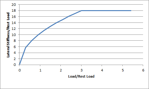
A good starting value for mLatStiffX is somewhere between 2 and 3. A good starting value for mLatStiffY is around 18 or so.

mFrictionVsSlipGraph[0][0]:

mFrictionVsSlipGraph[0][1]:

mFrictionVsSlipGraph[1][0]:

mFrictionVsSlipGraph[1][1]:

mFrictionVsSlipGraph[2][0]:

mFrictionVsSlipGraph[2][1]:

These six values describe a graph of friction as a function of longitudinal slip. Vehicle tires have a complicated response to longitudinal slip and this graph attempts to quickly describe this relationship.

Typically, tires have a linear response at small slips. This means that when the tire is only slightly slipping it is able to generate a response force that grows as the slip increases. At greater values of slip, the force can actually start to decrease from the peak value that occurs at the optimum slip. Beyond the optimum slip the tire eventually stops behaving less and less efficiently and hits a plateau of inefficiency.

The first two values describe the friction at zero tire slip: mFrictionVsSlipGraph[0][0] = 0, and mFrictionVsSlipGraph[0][1] = friction at zero slip.

The next two values describe the optimum slip and the friction at the optimum slip: mFrictionVsSlipGraph[1][0] = optimum slip, mFrictionVsSlipGraph[1][1] = friction at optimum slip.

The last two values describe the slip at which the plateau of inefficiency begins and the value of the friction available at the plateau of inefficiency: mFrictionVsSlipGraph[2][0] = slip at the start of the plateau of inefficiency, mFrictionVsSlipGraph[2][1] = the friction available at the plateau of inefficiency.

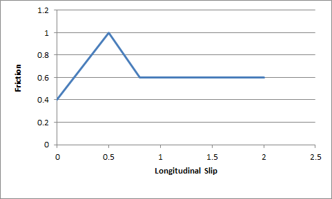
The friction values described here are used to scale the friction of the ground surface. This means they should be in range (0,1) but this is not a strict requirement. Typically, the friction from the graph would be close to 1.0 in order to provide a small correction to the ground surface friction.

A good starting point for this is a flat graph of friction vs slip with these values:

mFrictionVsSlipGraph[0][0]=0.0

mFrictionVsSlipGraph[0][1]=1.0

mFrictionVsSlipGraph[1][0]=0.5

mFrictionVsSlipGraph[1][1]=1.0

mFrictionVsSlipGraph[2][0]=1.0

mFrictionVsSlipGraph[2][1]=1.0

mCamberStiffness:

This value is currently unused.

mType:

This parameter has been explained in Section Tire Friction on Drivable Surfaces.

PxVehicleEngineData

mPeakTorque:

This is the maximum torque that is ever available from the engine. This is expressed in Newton metres. A starting value might be around 600.

mMaxOmega:

This is the maximum rotational speed of the engine expressed in radians per second.

mDampingRateFullThrottle:

mDampingRateZeroThrottleClutchEngaged:

mDampingRateZeroThrottleClutchDisengaged:

These three values are used to compute the damping rate that is applied to the engine. If the clutch is engaged then the damping rate is an interpolation between mDampingRateFullThrottle and mDampingRateZeroThrottleClutchEngaged, where the interpolation is governed by the acceleration control value generated by the gamepad or keyboard. At full throttle mDampingRateFullThrottle is applied, while mDampingRateZeroThrottleClutchEngaged is applied at zero throttle. In neutral gear the damping rate is an interpolation between mDampingRateFullThrottle and mDampingRateZeroThrottleClutchDisengaged.

The three values allow a range of effects to be generated: good accceleration that isn't hampered by strong damping forces, tunable damping forces when temporarily in neutral gear during a gear change, and strong damping forces that will bring the vehicle quickly to rest when it is no longer being driven by the player.

Typical values in range (0.25,3). The simulation can become unstable with damping rates of 0.

mTorqueCurve:

This is a graph of peak torque versus engine rotational speed. Cars typically have a range of engine speeds that produce good drive torques, and other ranges of engine speed that produce poor torques. A skilled driver will make good use of the gears to ensure that the car remains in the "good" range where the engine is most responsive. Tuning this graph can have profound effects on gameplay.

The x-axis of the curve is the normalised engine speed; that is, the engine speed divided by the maximum engine speed. The y-axis of the curve is a multiplier in range (0,1) that is used to scale the peak torque.

PxVehicleGearsData

mNumRatios:

This is the number of the gears of the vehicle, including reverse and neutral. A standard car with 5 forward gears would, therefore, have a value of 7 after accounting for reverse and neutral.

mRatios:

Each gear requires a gearing ratio. Higher gear ratios result in more torque but lower top speed in that gear. Typically, the higher the gear, the lower the gear ratio. Neutral gear must always be given a value of 0, while reverse gear must have a negative gear ratio. Typical values might be 4 for first gear and 1.1 for fifth gear.

mFinalRatio:

The gear ratio used in the simulator is the gear ratio of the current gear multiplied by the final ratio. The final ratio is a quick and rough way of changing the gearing of a car without having to edit each individual entry. Further, quoted gearing values from manufacturers typically mention ratios for each gear along with a final ratio. A typical value might be around 4.

mSwitchTime:

The switch time describes how long it takes (in seconds) for a gear change to be completed. It is impossible to change gear immediately in a real car. Manual gears, for example, require neutral to be engaged for a short time before engaging the desired target gear. While the gear change is being completed the car will be in neutral. A good trick might be to penalise players that use an automatic gear box by increasing the gear switch time.

PxVehicleClutchData

mStrength:

This describes how strongly the clutch couples the engine to the wheels and how quickly differences in speed are eliminated by distributing torque to the engine and wheels.

Weaker values will result in more clutch slip, especially after changing gear or stamping on the accelerator. Stronger values will result in reduced clutch slip, and more engine torque delivered to the wheels.

This value is to be edited only for very fine tweaking of the vehicle. Some clutch slip can be attributed to the numerical issues in the simulation at large timesteps, while some is a natural consequence of driving the car in an overly aggressive manner. A value of 10 is a good starting point.

PxVehicleAckermannGeometryData

mAccuracy:

Ackermann correction allows better cornering by steering the left and right wheels with slightly different steer angles, as computed from simple trigonometry. In practice, it is impossible to engineer a steering linkage that will achieve the perfect Ackermann steering correction. This value allows the accuracy of the Ackermann steering correction to be controlled. Choosing a value of 0 completely disables Ackermann steer correction. A value of 1.0, on the other hand, achieves the impossible dream of perfect Ackermann correction.

mFrontWidth:

This is the distance in metres between the two front wheels.

mRearWidth:

This is the distance in metres between the two rear wheels.

mAxleSeparation:

This is the distance in metres between the centre of the front axle and the centre of the rear axle.

PxVehicleTireLoadFilterData

This is for very fine control of the handling, and corrects numerical issues inherent in simulations at large timesteps.

At large simulation timesteps the amplitude of motion of the suspension springs is larger than it would be in real-life. This is unfortunately unavoidable. A consequence of this oscillation is that the load on the tire is more variable than expected, and the available tire forces have more variability than expected. On a bumpy surface this could mean that the simulation lifts the wheel off the ground, while in reality it should have stayed on the ground and delivered turning force. This filter aims to correct this numerical problem by smoothing the tire load, and perhaps even allowing turning force when the wheel is off the ground.

A key concept is that of normalised tire loads. A normalised tire load is just the actual load divided by the load experienced when the vehicle is in its rest configuration. If a tire experiences more load than it does at rest then it has a normalised tire load greater than 1.0. Similarly, if a tire has less load than it does at rest then it has a normalised tire load less than 1.0. At rest, all tires obviously have a normalised tire load of exactly 1.0. Another key idea is that when the wheel is just off the ground it can have a small negative load. Now, negative loads are a rather artificial result of the modelling mathematics and should be neglected entirely, but as already discussed, it might be beneficial to produce some tire force even when the tire is off the ground.

The values here describe points on a 2d graph that generates filtered tire loads from raw tire loads. The x-axis of the graph is "normalised tire load", while the y-axis of the graph is "filtered normalised tire load". Normalised loads less than mMinNormalisedLoad produce a filtered normalised load of 0. Normalised loads greater than mMaxNormalisedLoad produce a filtered normalised load of mMaxFilteredNormalisedLoad. Load in-between mMinNormalisedLoad and mMaxNormalisedLoad produce a filtered normalised load in-between 0 and mMaxNormalisedLoad, as computed by direct interpolation.

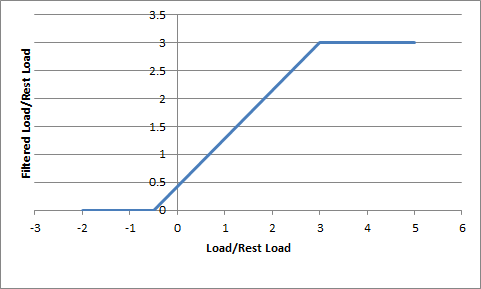
Choosing negative values for mMinNormalisedLoad results in small turning forces even when the tire is slightly off the ground. Additionally, choosing mMaxNormalisedLoad and mMaxFilteredNormalisedLoad limits the maximum load that will ever be used in the simulation. To disable the correcting effect of this graph choose mMinNormalisedLoad=0, mMaxNormalisedLoad=1000, and mMaxFilteredNormalisedLoad=1000.

PxVehicleDifferential4WData

mType:

A number of differential types are supported: 4-wheel drive with open differential, 4-wheel drive with limited slip, front-wheel drive with open differential, front-wheel drive with limited slip, rear-wheel drive with open differential, rear-wheel drive with limited slip.

mFrontRearSplit:

If a 4-wheel drive differential is chosen (open or limited slip) this option allows the drive torque to be split unevenly between the front and rear wheels. Choosing a value of 0.5 delivers an equal split of the torque between the front and rear wheels; that is, the total torque delivered to the front wheels is equal to the total torque delivered to the rear wheels. Choosing a value greater than 0.5 delivers more torque to the front wheels, while choosing a value less than 0.5 delivers more torque to the rear wheels. This value is ignored for front-wheel drive and rear-wheel drive differentials.

mFrontLeftRightSplit:

This is similar to the Front Rear Split but instead splits the torque that is available for the front wheels between the front-left and front-right wheels. A value greater than 0.5 delivers more torque to the front-left wheel, while a value less than 0.5 delivers more torque to the front-right wheel. This parameter can be used to prevent any torque being delivered to a damaged or disabled wheel. This value is ignored for rear-wheel drive.

mRearLeftRightSplit:

This is similar to mFrontLeftRightSplit except that it applies to the rear wheels instead of the front wheels. This value is ignored for front-wheel drive.

mFrontBias:

Limited slip differentials work by only allowing a certain difference in wheel rotation speed to accumulate. This prevents the situation where one wheel is slipping but ends up taking all the available power. Further, by allowing a small difference in wheel rotation speed to accumulate it is possible for the vehicle to easily corner by permitting the outside wheel to rotate quicker than the inside wheel.

This parameter describes the maximum difference in wheel rotation speed that is allowed to accumulate. The front bias is the maximum of the two front-wheel rotation speeds divided by the minimum of the two front-wheel rotation speeds. When this ratio exceeds the value of the front bias the differential diverts torque from the faster wheel to the slower wheel in an attempt to preserve the maximum allowed wheel rotation speed ratio.

This value is ignored except for front-wheel drive or four wheel drive with limited slip.

A good starting value is around 1.3.

mRearBias:

This is similar to mFrontBias except that it refers to the rear wheels.

This value is ignored except for rear-wheel drive or four wheel drive with limited slip.

A good starting value is around 1.3.

mCentreBias:

This value is similar to the mFrontBias and mRearBias, except that it refers to the sum of the front wheel rotation speeds and the sum of the rear wheel rotation speeds.

This value is ignored except for four wheel drive with limited slip.

A good starting value is around 1.3.

PxRigidDynamic

Moment of Inertia:

The moment of inertia of the rigid body is an extremely important parameter when editing vehicles because it affects the turning and rolling of the vehicle.

A good starting point for the moment of inertia of the rigid body is to work out the moment of inertia of the cuboid that bounds the chassis geometry. If the bounding cuboid is W wide, H high, and L long then the moment of inertia for a vehicle of mass M is:

((L*L+H*H)*M/12, (W*W+L*L)*M/12, (H*H+W*W)*M/12)

However, this is only a rough guide. Tweaking each value will modify the motion around the corresponding axis, with higher values making it harder to induce rotational speed from tire and suspension forces.

Providing unphysical values for the moment of inertia will result in either very sluggish behaviour or extremely twitchy and perhaps even unstable behaviour. The moment of inertia must at least approximately reflect the length scales of the suspension and tire force application points.

This parameter should be viewed as one of the first go-to editable values.

Center of mass:

Along with the moment of inertia, the center of mass is one of the first go-to editable values and, as such, has a profound effect on handling.

To discuss the center of mass it is useful to consider a typical 4-wheeled vehicle with a chassis mesh whose origin is at the centre of the four wheels. There is no requirement on the origin being at the center of the four wheels but it does make the following discussion a little simpler. It might be expected that the center of mass lies somewhere near this origin because vehicles are designed in a way that spreads the load almost evenly between the four wheels. More specifically, it might be expected that the center of mass needs to be a little above the base of the chassis rather than at the height of the wheels. After all, vehicles have higher mass density near the bottom of the chassis due to density of the engine and other mechanical systems. As a consequence, it is expected that the center of mass is nearer the bottom of the chassis than the top, but definitely above the bottom. Without a particularly detailed analysis of the chassis density distribution the exact location along the vertical axis is really a little arbitrary and subjective. Along the forward direction it might be expected that the center of mass is a little nearer the front wheels than the rear wheels because of the mass of the front-located engine. Thinking about these factors allows the center of mass to be tweaked along the vertical and forward directions.

Tweaking the center of mass is really all about making incremental changes that tune the handling towards a desired goal. Moving the center of mass forwards should help cornering because more load is distributed to the front tires. However, this comes at the expense of reduced load on the rear tires, meaning that the car might turn more quickly only to spin out because the rear tires lose grip more quickly. Small changes followed by tests on the handling are required.

When setting the center of mass it is important to bear in mind that the suspension sprung mass values might require simultaneous updating. If the center of mass moves nearer the front this means that more mass is supported by the front suspensions and less by the rear suspensions. This change needs to be reflected in a consistent way. It is possible to mathematically describe the relationship between center of mass and the mass split between the suspensions. However, the editing possibilities afforded by breaking this rigid link should allow more tweaking options.

Mass:

A typical car might have a mass of around 1500kg.