Joints
Joint Basics
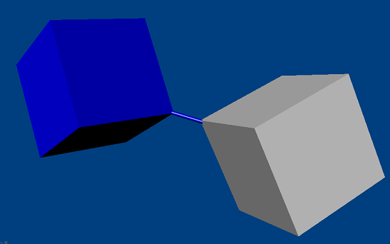
A joint constrains the way two actors move relative to one another. A typical use for a joint would be to model a door hinge or the shoulder of a character. Joints are implemented in the PhysX extensions library and cover many common scenarios, but if you have use cases that are not met by the joints packaged with PhysX, you can implement your own. Since joints are implemented as extensions, the pattern for creating them is slightly different from other PhysX objects.
To create a joint, call the joint's creation function:
PxRevoluteJointCreate(PxPhysics& physics,
                      PxRigidActor* actor0, const PxTransform& localFrame0,
                      PxRigidActor* actor1, const PxTransform& localFrame1);
This has the same pattern for all joints: two actors, and for each actor a constraint frame.
One of the actors must be movable, either a PxRigidDynamic or a PxArticulationLink. The other may be of one of those types, or a PxRigidStatic. Use a NULL pointer here to indicate an implicit actor representing the immovable global reference frame.
Each localFrame argument specifies a constraint frame relative to the actor's global pose. Each joint defines a relationship between the global positions and origins of the constraint frames that will be enforced by the PhysX constraint solver. In this example, the revolute joint constrains the origin points of the two frames to be coincident and their x-axes to coincide, but allows the two actors to rotate freely relative to one another around this common axis.
PhysX supports six different joint types:
- a fixed joint locks the orientations and origins rigidly together
- a distance joint keeps the origins within a certain distance range
- a spherical joint (also called a ball-and-socket) keeps the origins together, but allows the orientations to vary freely.
- a revolute joint (also called a hinge) keeps the origins and x-axes of the frames together, and allows free rotation around this common axis.
- a prismatic joint (also called a slider) keeps the orientations identical, but allows the origin of each frame to slide freely along the common x-axis.
- a D6 joint is a highly configurable joint that allows specification of individual degrees of freedom either to move freely or be locked together. It can be used to implement a wide variety of mechanical and anatomical joints, but is somewhat less intuitive to configure than the other joint types. This joint is covered in detail below.
All joints are implemented as plugins to the SDK through the PxConstraint class. A number of the properties for each joint are configured using the PxConstraintFlag enumeration.
Note: As in the rest of the PhysX API, all joint angles for limits and drive targets are specified in radians
Visualization
All standard PhysX joints support debug visualization. You can visualize the joint frames of each actor, and also any limits the joint may have.
By default, joints are not visualized. To visualize a joint, set its visualization constraint flag and the appropriate scene-level visualization parameters:
scene->setVisualizationParameter(PxVisualizationParameter::eJOINT_FRAMES, 1.0f);
scene->setVisualizationParameter(PxVisualizationParameter::eJOINT_LIMITS, 1.0f);

...

joint->setConstraintFlag(PxConstraintFlag::eVISUALIZATION)
Force Reporting
The joint may be configured to report each frame the force that was required to hold it together. To enable this behavior, set the joint's reporting flag. The force may then be retrieved after simulation with a call to getForce():
joint->setConstraintFlag(PxConstraintFlag::eREPORTING)
...

scene->fetchResults(...)
joint->getgetConstraint().getForce(force, torque);
The force is resolved at the origin of actor1's joint frame.
Note that this force is only updated while the joint's actors are awake.
Breakage
All of the standard PhysX joints can be made breakable. A maximum breaking force and torque may be specified, and if the force or torque required to maintain the joint constraint exceeds this threshold, the joint will break. Breaking a joint generates a simulation event (see PxSimulationEventCallback::onJointBreak), and the joint no longer partakes in simulation, although it remains attached to its actors until it is deleted.
By default the threshold force and torque are set to FLT_MAX, making joints effectively unbreakable. To make a joint breakable, specify the force and torque thresholds.
joint->setBreakForce(100.0f, 100.0f);
A constraint flag records whether a joint is currently broken:
bool broken = (joint->getConstraintFlags() & PxConstraintFlag::eBROKEN) != 0;
Breaking a joint causes a callback via PxSimulationEventCallback::onConstraintBreak. In this callback, a pointer to the joint and its type are specified in the externalReference and type field of the PxConstraintInfo struct. If you have implemented your own joint types, use the PxConstraintInfo::type field to determine the dynamic type of the broken constraint. Otherwise, simply cast the externalReference to a PxJoint:
class MySimulationEventCallback
{
    void onConstraintBreak(PxConstraintInfo* constraints, PxU32 count)
    {
        for(PxU32 i=0; i<count; i++)
        {
                        PxJoint* joint = reinterpret_cast<PxJoint*>(constraints[i].externalReference);
                            ...
        }
    }
}
Projection
Under stressful conditions, PhysX' dynamics solver may not be able to accurately enforce the constraints specified by the joint. PhysX provides kinematic projection which tries to bring violated constraints back into alignment even when the solver fails. Projection is not a physical process and does not preserve momentum or respect collision geometry. It is best avoided if practical, but can be useful in improving simulation quality where joint separation results in unacceptable artifacts.
By default projection is disabled. To enable projection, set the linear and angular tolerance values beyond which a joint will be projected, and set the constraint projection flag:
joint->setProjectionLinearTolerance(0.1f);
joint->setConstraintFlag(PxConstraintFlag::ePROJECTION, true);
Very small tolerance values for projection may result in jittering around the joint.
Limits
Some PhysX joints constrain not just relative rotation or translation, but can also enforce limits on the range of that motion. For example, in its initial configuration the revolute joint allows free rotation around its axis, but by specifying and enabling a limit, lower and upper bounds may be placed upon the angle of rotation.
Limits are a form of collision, and like collision of rigid body shapes, stable limit behavior requires a contactDistance tolerance specifying how close to the limit the joint configuration may be before the solver tries to enforce it. A high tolerance makes the limit less likely to be violated even at high relative velocity, but because the limit is active more of the time, the joint is more expensive to simulate.
Limit configuration is specific to each type of joint. To set a limit, configure the limit geometry and set the joint-specific flag indicating that the limit is enabled:
revolute->setLimit(PxJointLimitPair(-PxPi/4, PxPi/4, 0.1f)); // upper, lower, tolerance
revolute->setRevoluteJointFlag(PxRevoluteJointFlag::eLIMIT_ENABLED, true);
Limits may be either hard or soft. When a hard limit is reached, relative motion will simply stop dead (or, if you configure the limit with non-zero restitution, it will bounce.) When a soft limit is violated, the solver will pull the joint back towards the limit using a spring specified by the limit's spring and damping parameters. By default, limits are hard and without restitution, so when the joint reaches a limit motion will simply stop. To specify softness for a limit, declare the limit structure and set the spring and damping parameters directly:
PxJointLimitPair limitPair(-PxPi/4, PxPi/4, 0.1f));
limitPair.spring = 100.0f;
limitPair.damping = 20.0f;
revolute->setRevoluteJointLimit(limitPair);
revolute->setRevoluteJointFlag(PxRevoluteJointFlag::eLIMIT_ENABLED, true);
Note: Limits are not projected.
Actuation
Some PhysX joints may be actuated by a motor or a spring implicitly integrated by the PhysX solver. While driving simulations with actuated joints is more expensive than simply applying forces, it can provide much more stable control of simulation. See the specific documentation on the D6 and revolute joints for details
Note: The force generated by actuation is not included in the force reported by the solver, nor does it contribute towards exceeding the joint's breakage force threshold.
Fixed Joint
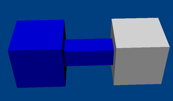
The fixed joint constrains two objects so that the positions and orientations of their constraint frames are the same.
Note
All joints are enforced by the dynamics solver, so although under ideal conditions the objects will maintain their spatial relationship, there may be some drift. A common alternative, which is cheaper to simulate and does not suffer from drift, is to construct a single actor with multiple shapes. However fixed joints are useful, for example, when a joint must be breakable or report its constraint force.
Spherical Joint
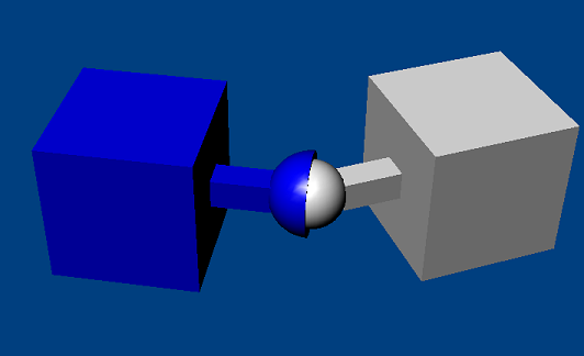
A spherical joint constrains the origins of the actor's constraint frames to be coincident.
The spherical joint supports a cone limit, which constrains the angle between the X-axes of the two constraint frames. Actor1's X-axis is constrained by a limit cone whose axis is is the x-axis of actor0's constraint frame. The allowed limit values are the maximum rotation around the the y- and z- axes of that frame. Different values for the y- and z- axes may be specified, in which case the limit takes the form of an elliptical angular cone:
joint->setLimitCone(PxJointLimitCone(PxPi/2, PxPi/6, 0.01f);
joint->setSphericalJointFlag(PxSphericalJointFlag::eLIMIT_ENABLED, true);
Note that very small or highly elliptical limit cones may result in solver jitter.
Note
Visualization of the limit surface can help considerably in understanding its shape.
Revolute Joint
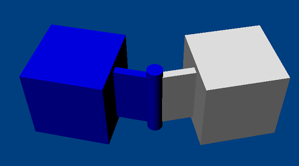
A revolute joint removes all but a single rotational degree of freedom from two objects. The axis along which the two bodies may rotate is specified by the common origin of the joint frames and their common x-axis. In theory, all origin points along the axis of rotation are equivalent, but simulation stability is best in practice when the point is near where the bodies are closest.
The joint supports a rotational limit with upper and lower extents. The angle is zero where the y- and z- axes of the joint frames are coincident, and increases moving from the y-axis towards the z-axis:
joint->setLimit(PxJointLimitPair(-PxPi/4, PxPi/4, 0.01f);
joint->setRevoluteJointFlag(PxRevoluteJointFlag::eLIMIT_ENABLED, true);
The joint also supports a motor which drives the relative angular velocity of the two actors towards a user-specified target velocity. The magnitude of the force applied by the motor may be limited to a specified maximum:
joint->setDriveVelocity(10.0f);
joint->setRevoluteJointFlag(PxRevoluteJointFlag::eDRIVE_ENABLED, true);
By default, when the angular velocity at the joint exceeds the target velocity the motor acts as a brake; a freespin flag disables this braking behavior.
Prismatic Joint
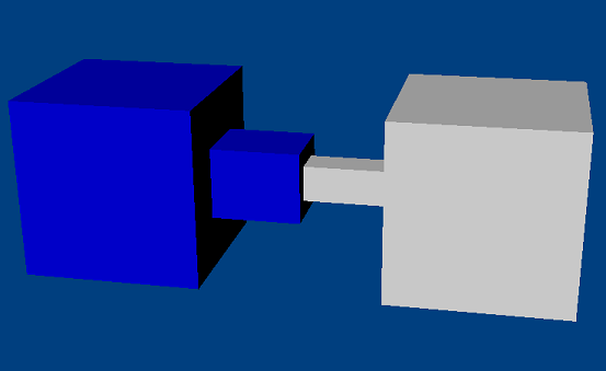
A prismatic joint prevents all rotational motion, but allows the origin of actor1's constraint frame to move freely along the x-axis of actor0's constraint frame. The primatic joint supports a single limit with upper and lower bounds on the distance between the two constraint frames' origin points:
joint->setLimit(PxJointLimitPair(-10.0f, 20.0f, 0.01f);
joint->setPrismaticJointFlag(PxPrismaticJointFlag::eLIMIT_ENABLED, true);
Distance Joint
The distance joint keeps the origins of the constraint frames within a certain range of distance. The range may have both upper and lower bounds, which are enabled separately by flags:
joint->setMaxDistance(10.0f);
joint->setDistanceJointFlag(eMAX_DISTANCE_ENABLED, true);
In addition, when the joint reaches the limits of its range motion beyond this distance may either be entirely prevented by the solver, or pushed back towards its range with an implicit spring, for which spring and damping paramters may be specified.
D6 Joint
The D6 joint is by far the most complex of the the standard PhysX joints. In its default state it behaves like a fixed joint - that is, it rigidly fixes the constraint frames of its two actors. However, individual degrees of freedom may be unlocked to permit any combination of rotation around the x-, y- and z- axes, and translation along these axes.
Locking and Unlocking Axes
To unlock and lock degrees of freedom, use the joint's setMotion function:
d6joint->setMotion(PxD6Axis::eX, PxD6Motion::eFREE);
Unlocking translational degrees of freedom allows the origin point of actor1's constraint frame to move along a subset of the axes defined by actor0's constraint frame. For example, unlocking just the X-axis creates the equivalent of a prismatic joint.
Rotational degrees of freedom are partitioned as twist (around the X-axis of actor0's constraint frame) and swing (around the Y- and Z- axes.) Different effects are achieved by unlocking various combinations of twist and swing.
- if just a single degree of angular freedom is unlocked, the result is always equivalent to a revolute joint. It is recommended that if just one angular freedom is unlocked, it should be the twist degree, because the joint has various configuration options and optimizations that are designed for this case.
- if both swing degrees of freedom are unlocked but the twist degree remains locked, the result is a zero-twist joint. The x-axis of actor1 swings freely away from the x-axis of actor0 but twists to minimize the rotation required to align the two frames. This creates a kind of isotropic universal joint which avoids the problems of the usual 'engineering style' universal joint (see below) that is sometimes used as a kind of twist constraint. There is a nasty singularity at π radians (180 degrees) swing, so a swing limit should be used to avoid the singularity.
- if one swing and one twist degree of freedom are unlocked but the remaining swing is kept locked, a zero-swing joint results (often also called a universal joint.) If for example the SWING1 (y-axis rotation) is unlocked, the x-axis of actor1 is constrained to remain orthogonal to the z-axis of actor0. In character applications, this joint can be used to model an elbow swing joint incorporating the twist freedom of the lower arm or a knee swing joint incorporating the twist freedom of the lower leg. In vehicle applications, these joints can be used as 'steered wheel' joints in which the child actor is the wheel, free to rotate about its twist axis, while the free swing axis in the parent acts as the steering axis. Care must be taken with this combination because of anisotropic behavior and singularities (beware the dreaded gimbal lock) at angles of π/2 radians (90 degrees), making the zero-twist joint a better behaved alternative for most use cases.
- if all three angular degrees are unlocked, the result is equivalent to a spherical joint.
Three of the joints from PhysX 2 that have been removed from PhysX 3 can be implemented as follows:
The cylindrical joint (with axis along the common x-axis of the two constraint frames) is given by the combination:
d6joint->setMotion(PxD6Axis::eX,     PxD6Motion::eFREE);
d6joint->setMotion(PxD6Axis::eTWIST, PxD6Motion::eFREE);
the point-on-plane joint (with plane axis along the x-axis of actor0's constraint frame) is given by the combination:
d6joint->setMotion(PxD6Axis::eY,      PxD6Motion::eFREE);
d6joint->setMotion(PxD6Axis::eZ,      PxD6Motion::eFREE);
d6joint->setMotion(PxD6Axis::eTWIST,  PxD6Motion::eFREE);
d6joint->setMotion(PxD6Axis::eSWING1, PxD6Motion::eFREE);
d6joint->setMotion(PxD6Axis::eSWING2, PxD6Motion::eFREE);
the point-on-line joint (with axis along the x-axis of actor0's constraint frame) is given by the combination:
d6joint->setMotion(PxD6Axis::eX,      PxD6Motion::eFREE);
d6joint->setMotion(PxD6Axis::eTWIST,  PxD6Motion::eFREE);
d6joint->setMotion(PxD6Axis::eSWING1, PxD6Motion::eFREE);
d6joint->setMotion(PxD6Axis::eSWING2, PxD6Motion::eFREE);
Limits
Instead of specifying that an axis is free or locked, it may also be specified as limited. The D6 supports three different limits which may be used in any combination.
A single linear limit with only an upper bound is used to constrain any of the translational degrees of freedom. The limit constrains the distance between the origins of the constraint frames when projected onto these axes. For example, the combination:
d6joint->setMotion(PxD6Axis::eX, PxD6Motion::eFREE);
d6joint->setMotion(PxD6Axis::eY, PxD6Motion::eLIMITED);
d6joint->setMotion(PxD6Axis::eZ, PxD6Motion::eLIMITED);
d6joint->setLinearLimit(PxJointLimit(1.0f, 0.1f));
constrains the y- and z- coordinates of actor1's constraint frame to lie within the unit disc. Since the x-axis is unconstrained, the effect is to constrain the origin of actor1's constraint frame to lie within a cylinder of radius 1 extending along the x-axis of actor0's constraint frame.
The twist degree of freedom is limited by a pair limit with upper and lower bounds, identical to the limit of the revolute joint.
If both swing degrees of freedom are limited, a limit cone is generated, identical to the limit of the spherical joint. As with the spherical joint, very small or highly elliptical limit cones may result in solver jitter.
If only one swing degree of freedom is limited, the corresponding angle from the cone limit is used to limit rotation. If the other swing degree is locked, the maximum value of the limit is π radians (180 degrees). If the other swing degree is free, the maximum value of the limit is π/2 radians (90 degrees.)
Drives
The D6 has a linear drive model, and two possible angular drive models. The drive is a proportional derivative drive, which applies a force as follows:
force = spring * (targetPosition - position) + damping * (targetVelocity - velocity)
The drive model may also be configured to generate a proportional acceleration instead of a force, factoring in the masses of the actors to which the joint is attached. Acceleration drive is often easier to tune than force drive.
- The linear drive model for the D6 has the following parameters:
- target position, specified in actor0's constraint frame
- target velocity, specified in actor0's constraint frame
- spring
- damping
- forceLimit - the maximum force the drive can apply
- acceleration drive flag
The drive attempts to follow the desired position input with the configured stiffness and damping properties. A physical lag due to the inertia of the driven body acting through the drive spring will occur; therefore, sudden step changes will result over a number of time steps. Physical lag can be reduced by stiffening the spring or supplying a velocity target.
With a fixed position input and a zero target velocity, a position drive will spring about that drive position with the specified springing/damping characteristics:
// set all translational degrees free

d6joint->setMotion(PxD6Axis::eX, PxD6Motion::eFREE);
d6joint->setMotion(PxD6Axis::eY, PxD6Motion::eFREE);
d6joint->setMotion(PxD6Axis::eZ, PxD6Motion::eFREE);

// set all translation degrees driven:

PxD6Drive drive(10.0f, -20.0f, PX_MAX_F32, true);
d6joint->setDrive(PxD6JointDrive::eX, drive);
d6joint->setDrive(PxD6JointDrive::eY, drive);
d6joint->setDrive(PxD6JointDrive::eZ, drive);

//Drive the joint to the local(actor[0]) origin - since no angular dofs are free, the angular part of the transform is ignored

d6joint->setDrivePosition(PxTransform::createIdentity());
d6joint->setDriveVelocity(PxVec3::createZero());
Angular drive differs from linear drive in a fundamental way: it does not have a simple and intuitive representation free from singularities. For this reason, the D6 joint provides two angular drive models - twist and swing and SLERP (Spherical Linear Interpolation).
The two models differ in the way they estimate the path in quaternion space between the current orientation and the target orientation. In a SLERP drive, the quaternion is used directly. In a twist and swing drive, it is decomposed into separate twist and swing components and each component is interpolated separately. Twist and swing is intuitive in many situations; however, there is a singularity when driven to 180 degrees swing. In addition, the drive will not follow the shortest arc between two orientations. On the other hand, SLERP drive will follow the shortest arc between a pair of angular configurations, but may cause unintuitive changes in the joint's twist and swing.
The angular drive model has the following parameters:
- An angular velocity target specified relative to actor0's constraint frame
- An orientation target specified relative to actor0's constraint frame
- drive specifications for SLERP (slerpDrive), swing (swingDrive) and twist (twistDrive):
- spring - amount of torque needed to move the joint to its target orientation proportional to the angle from the target (not used for a velocity drive).
- damping - applied to the drive spring (used to smooth out oscillations about the drive target).
- forceLimit - maximum torque applied when driving towards a velocity target (not used for an orientation drive)
- acceleration drive flag. If this flag is set the acceleration (rather than the force) applied by the drive is proportional to the angle from the target.
Best results will be achieved when the drive target inputs are consistent with the joint freedom and limit constraints.
Note
if any angular degrees of freedom are locked, the SLERP drive parameters are ignored. If all angular degrees of freedom are unlocked, and parameters are set for multiple angular drives, the SLERP parameters will be used.
Configuring Joints for Best Behavior
The behavior quality of joints in PhysX is largely determined by the ability of the iterative solver to converge. Better convergence can be achieved simply by increasing the attributes of the PxRigidDynamic which controls the solver iteration count. However, joints can also be configured to produce better convergence.
- the solver can have difficulty converging well when where a light object is constrained between two heavy objects. Mass ratios of higher than 10 are best avoided in such scenarios.
- when one body is significantly heavier than the other, make the lighter body the second actor in the joint. Similarly, when one of the objects is static or kinematic (or the actor pointer is NULL) make the dynamic bodythe the second actor.
A common use for joints is to move objects around in the world. Best results are obtained when the solver has access to the velocity of motion as well as the change in position.
- if you want a very stiff controller that moves the object to specific position each frame, consider jointing the object to a kinematic actor and use the setKinematicTarget function to move the actor.
- if you want a more springy controller, use a D6 joint with a drive target to set the desired position and orientation, and control the spring parameters to increase stiffness and damping. In general, acceleration drive is much easier to tune than force drive.