Tutorial
This tutorial contains step-by-step instructions on how to use the provided example dataset with SOM Analyst in ArcMap. The source data set for this tutorial is provided with SOM Analyst and is located in its sub-folder named dat. The file named census.csv contains gender, age, race, and housing data for each U.S. population census between the years 1900 and 1990.
First, the data is converted from the comma separated file format (.csv) to the database file format (.dbf) so that normalizations can be performed. Second, the raw count data are normalized by state population counts. Third, every variable is normalized into a 0 to 1 range and the preprocessed data are then exported to the SOM input format. Using those input data, a SOM is trained in two stages. The input data are then projected onto the finished SOM. Finally, a number of visualizations are produced.
System Requirements
- Windows (any version)
- ArcGIS 9.3 (legacy toolboxes for ArcGIS 9.0-9.2 are provided, but untested)
- Python 2.5 (included in the default ArcGIS 9.3 installation)
Download
SOM Analyst is available for download from http://somanalyst.googlecode.com
Adding the Toolbox
Add the SOM Analyst Toolbox to ArcGIS.
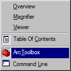
- Open the ArcToolbox panel by clicking on the Window menu and select ArcToolbox. Alternatively, click on the toolbox icon on the menu bar.
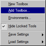
- Right click in the ArcToolbox panel and select Add Toolbox....
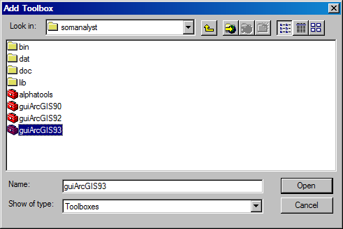
- Browse to the location of SOM Analyst and select guiArcGIS93.tbx and click Open.
Note
Depending on your computer setup, it may be necessary to first “connect” to the folder that contains SOM Analyst. In that case, click in the dialog box on the icon of a folder with an arrow pointing to a globe.
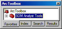
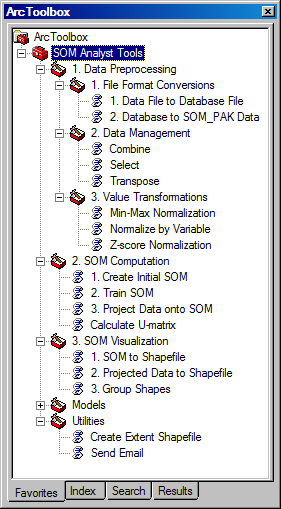
The SOM Analyst toolbox is now accessible through the ArcToolbox panel.
Browse through the toolbox to familiarize yourself with the tools.
Convert Data Format
Convert the data to a database file format.
- Run the Data File to Database File tool by double clicking on it in the File Format Conversions toolbox of the Data Preprocessing toolbox.
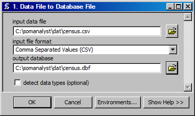
- Select census.csv as the input data file.
- Set Comma Separated Values (CSV) as the input file format.
- Change the output database file to census.dbf.
- Click OK to run the conversion.
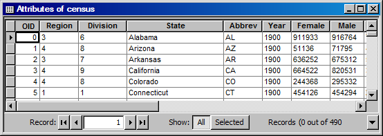
In the table properties the data type for each column is text.
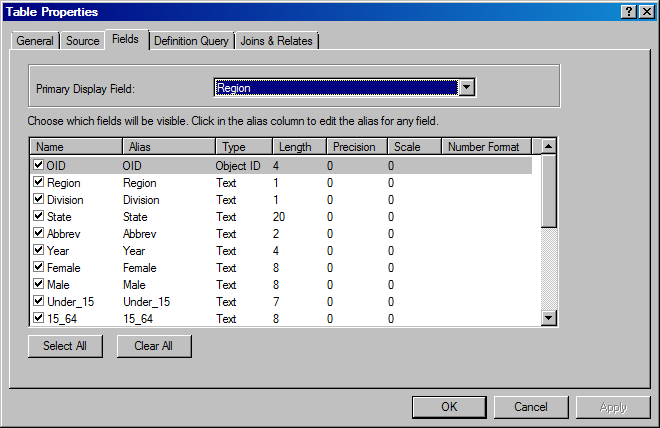
The values in the table are left justified indicating that they are text.
Normalize Data
Normalize values in the database file.
- Run the Normalize by Variable tool by double clicking on it in the Value Transformations toolbox of the Data Preprocessing toolbox.
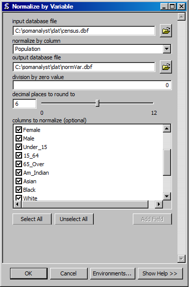
- Select census.dbf as the input database file.
- Select Population as the normalize by column.
- Change the output database file to census.dbf.
- Select the columns male, female, Under_15, 15_64, 65_Over, Am_Indian, Asian, Black, and White in the columns to normalize field.
- Click OK to run the normalization.
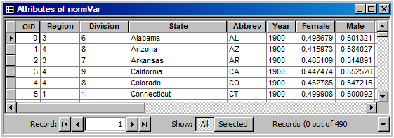
The resulting table contains population ratios.
- Run the Min-Max Normalization tool by double clicking on it in the Value Transformations toolbox of the Data Preprocessing toolbox.
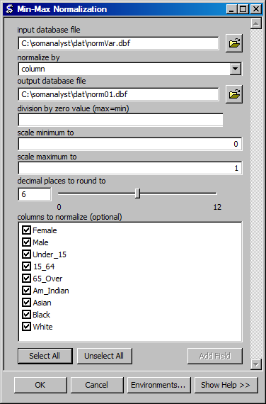
- Select normVar.dbf as the input database file.
- Select column as the normalize by field.
- Change the output database file to norm01.dbf.
- Select the columns male, female, Under_15, 15_64, 65_Over, Am_Indian, Asian, Black, and White in the columns to normalize field.
- Click OK to run the normalization.
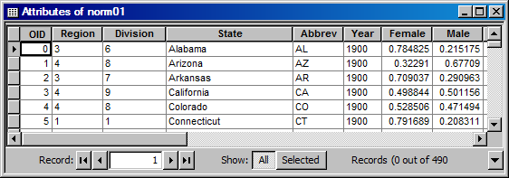
The resulting table contains normalized values.
Select Variables
Select the relevant variables from the database file.
- Run the Select tool by double clicking on it in the Data Management toolbox of the Data Preprocessing toolbox.
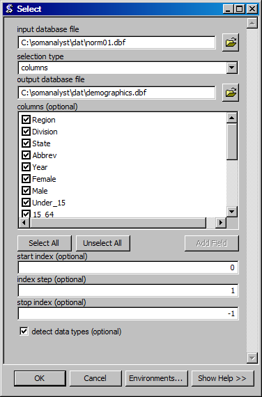
- Select norm01.dbf as the input database file.
- Set columns as the selection type.
- Change the output database file to demographics.dbf.
- Select all columns except Population, Owner, Renter, and Households in the columns field.
- Enable detect data types.
- Click OK to run the selection.
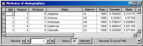
In table properties the value types for the columns has changed where appropriate.
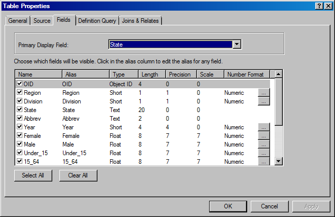
The numeric values in the table are right justified indicating that they are numbers.
Note
Detecting data types for columns requires checking the data type of each value and can be time consuming for large datasets. This step is only necessary if performing normalizations or other calculations before using the data with a SOM.
Export Data
Export the database file to the SOM data format.
- Run the Database File to SOM_PAK Data tool by double clicking on it in the File Format Conversions toolbox of the Data Preprocessing toolbox.
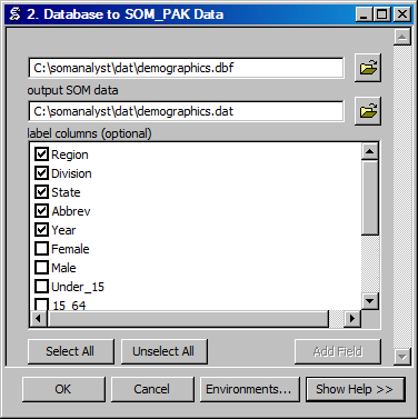
- Select demographics.dbf as the input database file.
- Change the output SOM data file to demographics.dat.
- Select Region, Division, State, and Year in the label columns field.
- Click OK to run the export.
Create Initial SOM
Creating the initial SOM.
- Run the Create Initial SOM tool by double clicking on it in the SOM Computation toolbox.
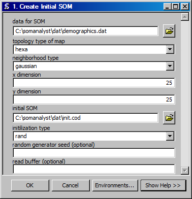
- Select demographics.dat as the data for SOM.
- Select hexa as the topology of map.
- Set 25 as the x dimension.
- Set 25 as the y dimension.
- Set init.cod as the initial SOM.
- Click OK to run the creation of the initial SOM.
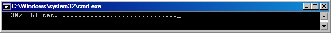
A window will open that indicates the progress of the process.
Train SOM
Training the SOM.
Note
The SOM will be trained in two steps. The first training will create the overall structure in the SOM. The second training will create the finer specialization.
- Run the Train SOM tool by double clicking on it in the SOM Computation toolbox.
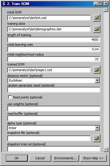
- Select init.cod as the initial som.
- Select demographics.dat as the training data.
- Set 4900 as the length of training.
- Set 0.04 as the initial learning rate.
- Set 25 as the initial neighborhood radius.
- Change the trained SOM to stage1.cod.
- Click OK to run the training of the SOM.
A window will open that indicates the progress of the process as it did with the creation of the initial SOM.
- Run the Train SOM tool.
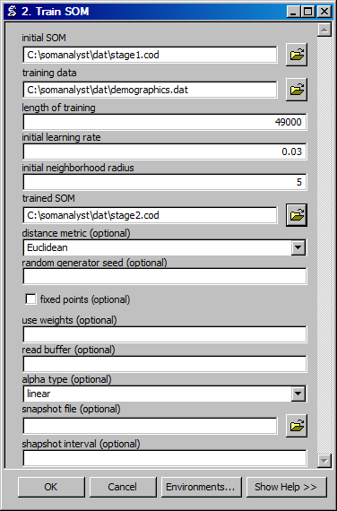
- Select stage1.cod as the initial som.
- Select demographics.dat as the training data.
- Set 49000 as the length of training.
- Set 0.03 as the initial learning rate.
- Set 5 as the initial neighborhood radius.
- Change the trained SOM to stage2.cod.
- Click OK to run the training of the SOM.
Calculate U-Matrix
Calculate the U-matrix of a SOM.
- Run the Calculate U-matrix tool by double clicking on it in the SOM Computation toolbox.
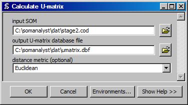
- Select stage2.cod as the input SOM.
- Change the output U-matrix database file to Umatrix.dbf.
- Click OK to calculate the U-matrix
Project Data onto SOM
Project the data onto the SOM.
- Run the Project Data onto SOM tool by double clicking on it in the SOM Computation toolbox.
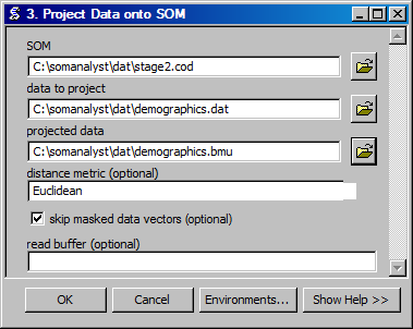
- Select stage2.cod as the SOM.
- Select demographics.dat as the data to project.
- Change the projected data to demographics.bmu.
- Click OK to project the data onto the SOM.
A window will open that indicates the progress of the process as it did with the creation of the initial SOM.
Create SOM Shapefile
Creating the SOM shapefile.
- Run the SOM to Shapefile tool by double clicking on it in the SOM Visualization toolbox.
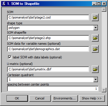
- Select stage2.cod as the SOM.
- Select polygon as the shape type.
- Change the SOM shapefile to stage2.shp.
- Set demographics.dat as the SOM data for variable names.
- Enable label SOM with data labels
- Set Umatrix.dbf as the U-matrix.
- Click OK to create the SOM shapefile.
Create Data Shapefile
Creating the data shapefile.
- Run the Projected Data to Shapefile tool by double clicking on it in the SOM Visualization toolbox.
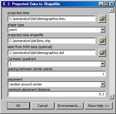
- Select demographics.bmu as the projected data.
- Select point as the shape type.
- Change the projected data shapefile to bmu.shp.
- Select demographics.dat as the label from SOM data.
- Select random around center as the placement.
- Click OK to create the data shapefile.
Group Data Shapefile
Grouping the shapes in the data shapefile.
- Run the Group Shapes tool by double clicking on it in the SOM Visualization toolbox.
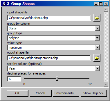
- Select bmu.shp as the input shapefile.
- Select State as the group by column
- Select polyline as the group type.
- Select maximum as the value type.
- Change the output shapefile to trajectories.shp.
- Select Year as the sort by column.
- Click OK to create the trajectories.
Create Extent Shapefile
Creating the extent shapefile.
- Run the Create Extent Shapefile tool by double clicking on it in the Utilities toolbox.
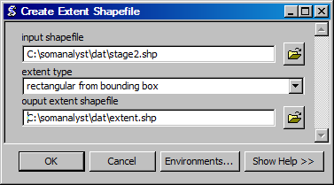
- Select stage2.shp as the input shapefile.
- Change the output shapefile to extent.shp.
- Click OK to create the extent shapefile.
Visualization
Visualizing the SOM and projected data.
- Open tutorial.mxd.
Note
Your map will not be identical, but should be very similar. The frames may appear rotated due to the initial random numbers used.
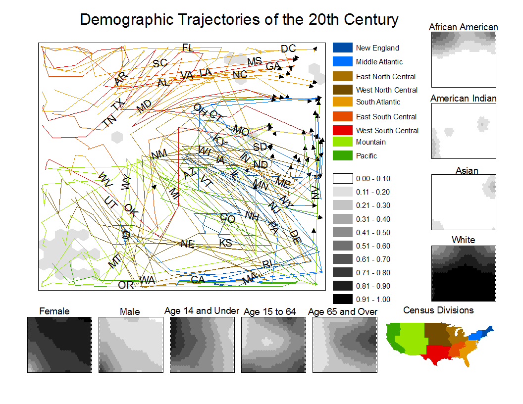
The large map shows the trajectory of each state across the SOM over time with a base of the U-matrix, a measure of distortion. The trajectories are color coded by census division, which are shown in the lower right. The other frames contain the component planes, each showing the neuron weights for one variable across the entire SOM.
When examining the demographic trajectories of each state note that each shift in the trajectory corresponds to a census year and that at the end of the trajectory is an arrow that represents the year 1990. Parallel trajectories indicate a similar change in demographics over time. Parallel trajectories are particularly evident within the South Division (West South Central Region, East South Central Region, and South Atlantic Region) and Northeast Division (Middle Atlantic Region and New England Region). This demonstrates spatial autocorrelation and is consistent with the demographic changes over the last century. In the Northeast Division, the parallel trajectories split 40 years ago mainly into coastal and land locked areas with New York and New Jersey similar to each other, but dissimilar to the other coastal states.
When examining component planes you are seeing how the SOM allocates location based on that variable. In this map, darker color means high values and lighter color means low values. You can see that the female component plane is very dark in one corner and light in the opposite corner with a gradual change between the two. Conversely the male component plane is very dark in the opposite corner and has a similar pattern of gradual change. When comparing component planes to each other you can see how the SOM weights the variables in the same location and thus derive a relationship between them. You can see that that female and male have an inversely proportional relationship in the SOM that corresponds with reality, that is that a high number of females inherently means a low number of males and vice versa.