Zooming and panning
From Matlab plt

Zooming and panning
Panning
The simplest way to pan the x or y axis is to click on one of the axis tick labels (actually anywhere outside the plot area will work) and drag it until the part of the display you wish to view is visible. Sometimes you may want to pan both the x and y axes at the same time. Instead of doing separate pans on each axis you can do both at the same time by clicking anywhere in the plot area (but NOT on any of the traces) and dragging that point until the desired view is achieved. Yet another way to pan the x axis is to use the optional x-axis cursor slider that is described in the next section (cursoring) One panning issue you should be aware of is that its performance will suffer when plotting very large arrays. For example, try the following command:plt(humps((1:1e6)/1e6)'*(1:4));
This will plot 4 traces each of which contains a million points. (These vectors are far bigger than what you will usually want to plot.) The display update rate while panning this plot on my 2011 era desktop computer is about 3 times per second, which is noticeably jerky but certainly useable. However if you want to plot even more data than this it may make sense to decimate it before plotting. Your eye won't know the difference by the time you are plotting more than a couple of hundred points per trace, so you won't really be missing anything unless you zoom in dramatically.
Zooming
Try the same thing as with panning, except drag with the right mouse button instead of the left. You will find that dragging towards the origin compresses the axis (for zooming out) and dragging away from the origin expands the axis (for zooming in). As with panning you can zoom both axes at once by a right click and drag in the plot area. (Unlike panning you don't have to worry about whether you are on a trace or not. The same thing will happen in either case.)Often to get the desired view requires two mouse movements. The first, with a right click and drag to expand or contract the axis (or axes) and the second, with a left click, to re-center the display. You may find that this is the most convenient method, or perhaps you will like one of the seven other methods described below.
The expansion box
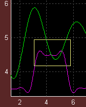 If the portion of the graph that you want to zoom in on is completely visible
on the graph, the fastest way to display the desired area is to draw an
expansion box. This is the way you will likely use most often, so you should try
all four ways to draw the expansion box that are listed below to see which ones
you like best.
If the portion of the graph that you want to zoom in on is completely visible
on the graph, the fastest way to display the desired area is to draw an
expansion box. This is the way you will likely use most often, so you should try
all four ways to draw the expansion box that are listed below to see which ones
you like best.
- Position the mouse in the plot area over one corner of the area you wish to zoom in on. Then click both mouse buttons at the same time, holding them both down while dragging the mouse towards the opposite corner of the desired zoom area. A yellow box will be drawn, which will be stretched or contracted as you drag the mouse around. When you let go of the mouse, the display will look similar to the picture to the left.
- An alternate method which you may find easier is double click the left mouse button, but don't release the button after the second click. Hold the mouse button down while you drag to create the expansion box.
- A method which requires less coordination is to press and hold the keyboard shift key, then click and drag with the mouse until the expansion box is the size you want.
- And finally you can left-click the grey "x" label in front of the x-cursor edit box. (Actually using the grey "y" label in front of the y-cursor edit box does exactly the same thing.) This draws the expansion box covering the exact same area as the current axis limits, and then zooms the display out by about 20% so that you can see the expansion box. This method makes more sense when you which to make small changes to the x or y axis limits or when you are planning to type in the new limits numerically.
If plt was called with the MotionZoom or the MotionZup parameter, the function specified with that parameter can cause additional text, plots or other visual effects to appear and be modified as you adjust the size of the expansion box. (See Mouse Motion Functions)
Accepting or cancelling the limits indicated by the expansion box
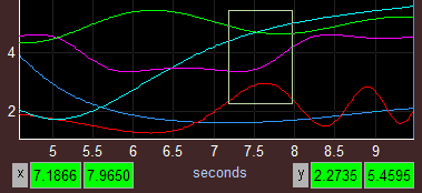 After an expansion box is drawn using any of the four methods described above,
both the x and y-cursor edit boxes double up and contain the limits of the expansion box
(as shown in this figure). To accept the current limits shown, simply LEFT
click anywhere inside the plot area. To remove the expansion box keeping the axis
limits the way they were, simply right-click anywhere inside the plot area.
After an expansion box is drawn using any of the four methods described above,
both the x and y-cursor edit boxes double up and contain the limits of the expansion box
(as shown in this figure). To accept the current limits shown, simply LEFT
click anywhere inside the plot area. To remove the expansion box keeping the axis
limits the way they were, simply right-click anywhere inside the plot area.
You may want to modify the expansion box size or position before accepting it. Several methods of doing this are described below.
Adjusting the expansion box
The most precise way of setting the expansion box limits is to simply type them in. For example, suppose you want to change the x-limits shown in the figure above (7.1866 to 7.9650) to the values 7.1 to 7.9. Simply highlight the lower limit x limit (7.1866) by dragging the mouse over it and then type in the desired value (7.1). Then press "tab" which will accept that value and automatically highlight the next value (upper x-limit). Then after entering the upper limit, press tab again to highlight the y-axis lower limit ... or if you don't want to edit the y limits as well, hit enter instead of tab. As soon as you hit enter or tab each time you will see the edit box change in the plot area to reflect the entered values. Note that the limits are shown in increasing order, however you are not restricted by that convention. (i.e. entering the limits 4,3 draws the same expansion box as if you entered 3,4). Although this method is by far the most precise way to adjust the expansion box, it is usually more convenient to do this using the mouse as described below:- Adjusting the expansion box size
Simply click and drag on any of the four corners of the expansion box. The corner you clicked on will follow the mouse while the diagonally opposite corner will remain fixed. Note that the mouse behaves in the same way as when the expansion box was first drawn. - Adjusting the expansion box position (preserving its size)
Click on the midpoint of any edge of the expansion box and simply drag the expansion box to its desired location. The expansion box size does not change during this operation.
Alternate method
In earlier versions of plt (before the above method was devised) a different method was used to adjust the expansion box with the mouse. Although it allows you to adjust a single edge at a time (as well as moving the position while preserving size), you will probably find this older method less natural. Never-the-less I did not remove this method in case you became used to it with older versions of plt. Newer users will probably stick to the method described above, but for completeness the older method is described below:
- Right-click anywhere near the middle of the lower x limit (the 7.1866 number in this figure) but don't release the mouse button. As you are holding the mouse button down, drag the mouse to the left or the right. (You don't have to remain inside the edit box, or even inside the figure window for that matter). As you drag to the left you will see the 7.1866 number decreasing and also the left edge of the expansion box will move to the left. As you drag the mouse to the right of center, number will start increasing and the expansion box moves accordingly. The farther you drag the mouse from the center of the edit box, the faster the left edge of the zoom box moves. Any vertical movement of the mouse in this situation is ignored.
- Right-click anywhere near the middle of the upper x limit (the 7.9650 number in this figure), hold the mouse down and drag left or right. This time the right side of the edit box moves in a similar manner to that described above.
- Right-click near the middle of the lower y limit (the 2.2735 number) to adjust the lower edge of the expansion box in a similar manner except now only the vertical movement of the mouse matters. Any horizontal movement is ignored.
- Right-click near the middle of upper y limit (the 5.4595 number) to adjust the upper edge of the expansion box. Again, any horizontal movement is ignored.
- Note that the mouse methods for adjusting the four edges described so far alter the size of the expansion box. There is one final method to describe that doesn't change the size of the expansion box, but only its position. Right-click on the left or right edge of any of the four edit boxes, leaving the mouse button down while dragging the mouse as before. (You might have to be pretty close to one of these edges for this to work.) This time, as you drag, the position of the expansion box moves in the same direction as the mouse offset from the original clicked position. The farther the mouse is moved from this original position the faster the expansion box position changes. Unlike the previous four situations, here both the horizontal and vertical movements of the mouse have an effect, so you can even move the box's position diagonally if you choose. Note that the behavior is the same no matter which of the four edit boxes you use to initiate the action. The size of the expansion box will not change during this movement with one exception. If you bump the expansion box into one of the edges the box becomes smaller because the trailing edge will continue to move even after the leading edge has hit the wall.
Auto scaling
If plt is called without any 'xlim' or 'ylim' arguments, both axes are initially auto-scaled to show the entire data range. At any later time you can auto-scale the x-axis by right-clicking on the grey "x" label in front of the x-cursor edit box. Right clicking on the grey "y" label is similar for auto-scaling the y-axis, although there is one difference. The difference is that the y-axis is scaled to insure that the data associated with the active trace is visible. There is an alternate way to auto-scale that picks display limits to insure that all the traces are visible instead of just the active trace. (See "Expansion history" below).Expansion history
Whenever you change the x or y axis limits by any of the above methods, the previous limits are stored in a expansion history list. You can cycle through these stored limits by left-clicking on the XY↔ tag in the menu box. (See "Menu box" below). This list is 4 elements deep, so when you zoom or pan the fifth time the oldest display limits fall off the bottom of the stack. Assuming the expansion history list is full (which is usual) clicking on the XY↔ tag four times in a row will show you the last four display limits. On the fifth click, plt will auto-scale both the x and y axes in a way that insures that all the data for all traces falls inside the display area. On the sixth click, plt goes back to using the axis limits stored in the expansion history list. Although you can auto-scale by clicking on the XY↔ tag a suitable number of times that can be cumbersome since you usually don't know where you are in the rotation. For this reason a faster way to auto-scale is provided ... simply right click once on the XY↔ tag.Doubling or halving the display area
Left-clicking the Zout tag in the menu box (see "Menu box" below) expands each axis by 40% which increases the display area by 1.42 (1.96) i.e. approximately doubling the display area. Right-clicking zooms in, halving the display area. In both directions the center point of the display remains in the center after the zoom operation.xView slider
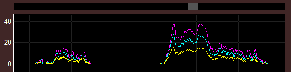
The black horizontal bar with the short gray segment that appears above the plot is called the xView slider. It provides yet another way of panning and zooming the x-axis and is particularly useful when you want to view a small segment of a long data set. The whole bar represents the entire data set and the gray segment represents the portion of the data currently in view. If 10% of the data is currently in view, then the length of the gray segment will be 1/10 the length of the whole bar. Similarly the position of the gray segment within the bar represents the position of the displayed data relative to the whole data set.
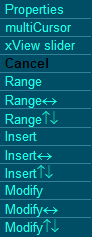
To bring up the xView slider, first right-click on the Ycursor edit box. This will bring up the Yedit popup menu shown here. Then select the third item in this menu (xView slider) and the slider will appear. This is a toggle, so selecting it again will make the xView slider disappear.
If you wanted to the xView slider to appear when your program starts up, you can include the string xView in the 'Options' parameter. Also you can enable or disable the xView slider from the command line or in a program with the command
Moving the gray segment left or right is as easy and natural as you would expect. Simply click on the gray segment and drag it left or right. The plot underneath will update as you are sliding allowing you to easily search for the data portion that interests you. You can also make the gray segment larger so that a larger portion of the data is displayed. To do this simply click in the black area to the left of the gray segment and the left edge of the gray segment will immediately be extended to the point where you clicked. (Similar for the right edge of course.) But notice that this method won't work if you want to make the gray segment smaller. So how do we do it? Simple, just click in the black area, hold down the mouse and drag. The edge that you selected will follow the mouse allowing you to place it wherever you want. (An alternate method of making the gray segment smaller is to right-click inside the gray segment, but the first method I mentioned is usually easier.) And finally there is one more trick you can do with the gray segment. Double clicking on it expands the gray segment to fill the entire black bar (i.e. it resets the x-axis limits to cover the full extent of the x data). This is somewhat similar to right-clicking on the menubox XY↔ tag except that the XYrotate tag effects both the x and y axis where as the xView slider never effects the y axis. (Double clicking on the gray segment a second time undoes the effect of the first double click.)
Notice that when the x-axis is zoomed or panned by any of the other methods provided, the xView slider will automatically be updated so that the gray segment properly represents the visible portion of the data.
The appearance of the xView cursor is probably suitable for most situations, but you can modify its appearance by using the xvProps figure application data. This is best illustrated with an example. Suppose we follow the call to plt with the expression:
setappdata(gcf,'xvProps', ...
{'color' 'red' '+color' 'blue' '+' [0 -.01 0 .02]});
The cell array consists of property name/value pairs. If the property name does not have the "+" prefix the property is applied to the short gray segment, so the first property pair above changes the gray segment into a red segment. If the property name does include a "+" prefix then the property is applied to the long horizontal black bar (which actually is an axis). So the second property pair changes the black bar into a blue one. Any axis property name may be used. The last property pair is a special case since it has the prefix without a property name. The meaning of this special case is that the value specified is to be added to current position value for the horizontal bar (axis). So what this example does is to move the (blue) horizontal bar down by 1% of the figure height and to make the bar thicker by 2% of the figure height. (Note that you could also specify the position in absolute terms be replacing the '+' with '+pos')