GUI building with plt

previous page next page

GUI building with plt

Over the years I have created dozens of GUIs using Matlab, nearly all of which involved collecting and/or viewing data and interacting with the data or data collection process in some way, and I suspect the same is true for the GUIs that you need to create. The first GUIs I created were quite difficult, but as I built up my bag of tools each new program became easier and quicker to write. The key I found was to avoid re-inventing the wheel each time and the best way to do that was to create a series of "pseudo objects". A pseudo object is a collection of Matlab graphics objects embedded with features commonly needed in Matlab GUI applications. (I chose to call them pseudo objects to distinguish them from the graphics objects supplied in the standard Matlab environment.) These pseudo objects are combined into one file exchange submission called (for historical reasons) plt. My primary goal for plt is to make building GUI applications in Matlab easier, faster, and more fun while enabling you to create clearer, more concise code that is compatible across all Matlab platforms and versions.

The two main tasks in creating a GUI application are:

Choosing the graphical elements and configuring the sizes and positions of these elements.
Writing the code that enables these graphical elements to serve their intended purpose.

Matlab's GUI building tool (called Guide) helps a lot with the first task but contributes little to the second. However I've found that for all but the most trivial applications, the second task accounts for most of the frustrations and time spent. My strategy is to aid the second task by providing a rich set of the pseudo objects mentioned above. It may seem like this is a tall order for these new objects, but I hope the examples that follow will convince you that they can impressively reduce the amount of code you need to write. The current set of pseudo objects is merely a start. I plan to continue implementing new pseudo objects ... hopefully many of them conceived by Matlab users such as yourself.

A parallel goal is to make it easier to learn Matlab GUI programming by providing many well commented examples that demonstrate as many of the pseudo object features as possible. It's easier to begin a new GUI application by starting with an example that has at least some of the graphical features that you need. To this end, plt includes 26 example programs covering a wide variety of GUI features and programming techniques. New example programs have been steadily added to the list over the years since the first version of plt, often initiated by questions and requests sent to me by plt users. Although the standard Matlab plotting and graphical elements are thoroughly documented, a common complaint is that this information is spread out over thousands of pages of Matlab documentation making it difficult to find what you are looking for. Also it is difficult to find examples for most features. This inspired me to design the plt help file to avoid these pitfalls by organizing plt's many features into one coherent help file including many examples. Every question from a plt user leads me to reexamine the documentation to see if I have described each feature and example as completely and clearly as possible.

Although the first task mentioned above (configuring sizes and positions of graphical elements) is not where most of the time is spent, without an appropriate tool this could be a painstaking task. Matlab's Guide tool does provide a reasonable solution to this problem however I found several annoyances with this tool:

Guide forces me to adopt a particular programming methodology and style. Although plt offers unique pseudo objects you are free to use all or none of them to suit your purpose and no demands are made on your programming style. My preferences lean towards conciseness and clarity, as you can see from my programming examples.
Guide has evolved over the years and works somewhat differently in different Matlab versions which can cause compatibility issues. I often support my Matlab applications for use with older Matlab versions, some of which were released even before Guide was invented.
I sometimes find it inconvenient that the program definition is split between the .m and .fig files. The .fig file format can also lead to Matlab version dependencies. (GUIs designed with plt don't depend on .fig files.)
And most importantly Guide was not compatible with the powerful pseudo objects that I had created.

In addition, to the Guide compatibility issues mentioned in point 2 above, the graphics objects themselves have changed between versions. For example the latest Matlab version (R2014b) finally allows you to set the grid line color independently allowing you to create far more pleasing plots. However this won't help when you try to run your program on previous Matlab versions (which in fact represent the majority of the user base). On the other hand, plt is designed to work the same across all Matlab versions, so you can share your code with colleagues running older Matlab versions. I have tested plt on most Matlab releases dating as far back as June 2001 (Matlab 6.1) and of course it works with Matlab's most recent R2014b version as well. You might think that supporting older versions would limit plt's flexibility, however as you will see plt generally meets or exceeds the flexibility available with even the latest native Matlab plot commands (including grid lines of course).

After abandoning Guide for the above reasons, at first I simply entered position coordinates by hand, often iterating many times to adjust controls to achieve the desired look. But for complicated GUIs with many objects, this is too time consuming. This led me to develop a more automated method of positioning pseudo objects as well as native Matlab objects without using Guide. This method is not quite as automated as Guide, but I hope you will see from the following examples that it strikes a good balance between automation, power, and flexibility. The basic idea was to give plt the the ability to reposition and resize the graphical objects and to display the results in a way that allows you to copy the positions of all your objects into your program with a single cut and paste.

Since the pseudo objects are the key innovation that simplifies Matlab GUI programming, let's briefly summarize the nine pseudo objects that have been implemented so far:

Cursor - My goal for the cursor pseudo object was to tailor plt for its role in data exploration. The ease and responsiveness of the cursoring, panning, and zooming operations is unmatched by any other Matlab plotting package (at least according to reports from some plt users). Although you can create cursor pseudo objects independently, by default a cursor object is created for you when you define a plt pseudo object. This relieves you of the need to know about the many details of the cursor object.
Grid - In the latest Matlab release (R2014b) you can change the grid color using the axis 'gridcolor' property. However as I mentioned earlier, using this property will give an error if you run the program on any earlier Matlab release. If you are using any release earlier than R2014b, you can see the problem by typing plot(rand(1,100)); grid on;. and note how the grid lines are so overpowering it is hard to see the trace underneath. Now try changing the grid line color to something less overwhelming by typing set(gca,'xcolor',[.7 .7 .7],'ycolor',[.7 .7 .7]);. Now the grid lines look pretty nice but the tick labels become so faint you can barely see them. (This insanity was an annoyance and embarrassment to Matlab users for at least two decades and in fact was one of my motivations for creating the first version of plt a decade ago). The plt grid pseudo object gives you even more flexibility than the latest Matlab release by allowing you to select the grid color, thickness, line style, and erase mode without affecting any other graphic element. As with the cursor pseudo object, you will rarely need to define a grid pseudo object explicitly since it is also created by the plt pseudo object. The defaults are to most people's liking so you may never need to adjust them.
plt - This can be thought of a super axis (or collection of axes). In that respect it is similar to Matlab's plot and data is passed to plt in the same way making simple calls to plt look the same as the call to plot (except for the missing "o"). However unlike plot, plt also (by default anyway) creates:
- a cursor pseudo object.
- a grid pseudo object.
- a menu box containing various plotting controls.
- a TraceID box which serves both as a legend and as a way to enable and disable individual traces.
- a menu bar containing the traditional Matlab menus (File,Edit,View,Tools,etc) as well as a plt menu containing items unique to plt.
The plt pseudo object integrates all these elements together in a consistent logical manner with the defaults oriented towards the typical data exploration needs of the most common graphical interfaces. This allows you to take advantage of the plt features in your design even before learning about the many ways to tailor plt to your needs. It might seem strange that I use "plt" both as the name of this pseudo object as well as the name of the entire toolbox, however I think you will find that you can tell which one I'm referring to by context.
Slider - Matlab's slider is the most versatile uicontrol because of the many ways you can change the value (dragging the slider bar, clicking the left or right arrow, clicking the trough). Plus it is the only uicontrol whose action can repeat continuously as you hold down the mouse button. This allows you to smoothly vary a parameter over a range while observing its effect. However the slider control rarely can stand alone. At a minimum you need a label to identify what the control is for and usually you also need a more precise representation of the slider value than the slider bar itself provides. A text box is often used for this purpose, although an edit box is better since it allows a way to set the slider value precisely. It is also common to want labels to identify the minimum and maximum values associated with the left and right slider bar positions. Furthermore sometimes the slider value must be restricted to be an integer or a multiple of some other factor or other condition (such as a power of 2 for example). Also you may want to adjust the step size for the arrows or trough or to make the steps logarithmically spaced. These requirements mean that you usually need to write a lot of code to make a slider useful for your application. The pseudo slider solves this problem by integrating all the elements and options just mentioned into one object that you can simply drop into your application and move around as a unit. All the code you need to make it useful is already done for you!
Edit - As mentioned above, the ability of the slider and the pseudo slider to respond continuously as the mouse button is held down is a powerful feature. The one drawback of these objects is that they take up quite a bit of space. For a GUI with many controls, you may not have room to use sliders for many of them. The edit pseudo object is the answer to such a problem. It takes up even less space than a uicontrol edit box. It doesn't have all the features of the pseudo slider, but you can continuously increment its value by holding down the mouse on the right side of the object, and likewise decrement its value on the left side. Like the pseudo slider, you can select the increment amount as well as the min/max limits. The edit object may also be used to contain vectors or strings. (The auto-increment features do not apply in that case.) Usually edit objects require a label to identify the purpose of the control. The edit pseudo object includes a label (optionally) as an integrated feature. When you reposition the edit control, the label moves right along with it. One less graphical object to define, size, and position. Other advantages over the uicontrol edit box include:
- Auto evaluations
- More flexible formatting
- More powerful callbacks
- Tex interpreter support
- Choice of figure or axis coordinates
As an example of an Auto evaluation, consider that typing "cos(pi/6)" into the pseudo object would set its value to 0.866025 (with fewer or more digits depending on the format code). The last point also deserves elaboration. Normally you will want to define the edit pseudo object in figure coordinates (what I call a type I edit pseudo object) just as you do with a uicontrol. However if you want to associate the object with a plot (so it moves with the plot if it is repositioned, or if you want to create an array of edit objects it is more convenient to use axis coordinates (i.e. a type II edit pseudo object).
Popup - The popup pseudo object closely mimics the function of Matlab's popup uicontrol but has these advantages:
- You can fit twice as many pseudo popups into a given space as uicontrol popups.
- You can cycle through the popup's options without opening the popup by right clicking on the object. When you want to see the effect of all the possible selections, it is far faster with the pseudo popup than with the uicontrol.
- Optionally swap the role of left & right clicks (super-button mode).
- Integrated label (optional).
- More powerful callbacks.
- Independent control of the location/appearance of the opened and closed view of the popup.
- More flexible formatting.
- Tex interpreter support.
- Ability to open or close the popup from a program.
Of course uicontrol popups and uicontrol edit boxes may still be used and may be preferred when you don't need any of the advantages listed above.
Image - Most of plt's features are tailored toward 2D plotting (functions of a single variable). However plt provides two methods to plot functions of two variables. One is to use a waterfall plot which makes use of the auxiliary function pltwater.m. The other method is to use the Image pseudo object. The Image pseudo object provides cursoring methods appropriate for this object type and also includes several optional components including:
- A color bar which serves as a legend for the z-axis values as well as providing a method of changing the colormap used to represent the z data.
- A slider (labeled 'edge') that allows you to control how wide a range around a midpoint is used when determining the color used to represent each array element.
- A slider (labeled ''mid'') that allows you to control the center value of the range of values used to determine the color for each array element.
- A checkbox that allows you to control the visibility of the axis gridlines.
- A 'view all' button, that when clicked on resets the axis limits so that all the data is visible. A secondary feature of this button is activated by right-clicking on it instead which zooms in on the center of the region currently in view.
ColorPick - Nothing is quite as individual as the colors we prefer in our applications, and allowing the user to choose the application colors is a true sign that the programmer cares about the user. However choosing several colors that have to blend together in a pleasing way is not a simple matter and providing a substandard interface for color choice can be more of a curse than a blessing. The ColorPick pseudo object was carefully designed to make it as easy as possible to give your application this flexibility. I've found it is important to present the user with palettes of colors to choose from and have the selected objects change instantly when a new choice is made. A very simple example of the use of the ColorPick object is given in gui2.m. A more elaborate example is the demoplt.m program which also includes the code to save the selected colors in a setup file so that the chosen colors remain permanent until changed again.
HelpText - To make our GUIs as easy to use as possible, it is nice to show help messages right on the main GUI figure. Even if the GUI is complicated enough to need a manual, most people won't read it and even if they do, some reminders of the basics when the program starts up can be useful. Of course these reminders will quickly become annoying if they get in the way or take up valuable screen area that could be better used by the application. The HelpText pseudo object was designed to solve this need by making it easy to format and position the help messages as well as to make them disappear as soon as you start using the GUI. When this pseudo object is created along with the plt pseudo object (by using the 'HelpText' parameter), right-clicking on the menu box help tag will make the help text reappear, although it is easy to create a dedicated button for that purpose if you prefer.

A more complete description of these pseudo objects from a programming perspective can be found here: Pseudo objects.

Now you are prepared to dive into the examples that follow:

A first example

Our first GUI example doesn't do any plotting or anything else useful for that matter, so it may not present a compelling case for the GUI tools provided by plt. However since it consists of just a few dozen lines of code it is simple enough that you can quickly see how to use plt to arrange graphic elements inside a figure window.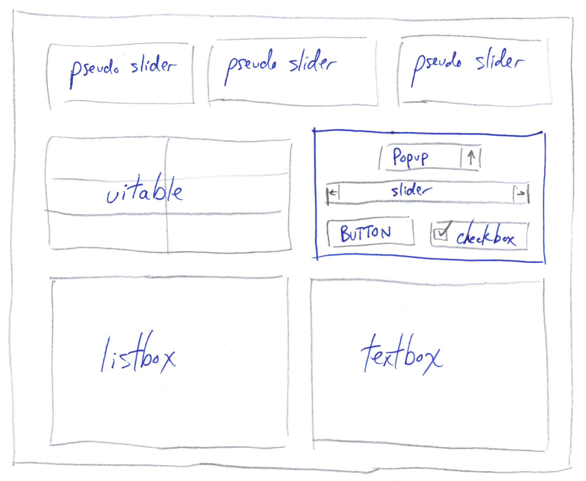

I find that it is best to start working on a new GUI with pencil and paper. Imagine the control types and arrangement for the application and then sketch a mock up such as this. Your finished application rarely will look much like your first sketch, but with the rapid prototyping possible with Matlab and plt you can quickly iterate improvements in form, concept and implementation.

Here I have decided on 3 pseudo sliders across the top followed below by a uitable on the left and a frame on the right containing 4 uicontrols (a popup, slider, button, and checkbox).

The bottom part of the GUI consists of two large objects for displaying lists of numbers. The right most one is a simple text box with room to show about 10 lines of text. The left most one is a listbox which by virtue of its scroll bar can display a far larger data set (80 lines of text in this example).

First we create the figure window. I usually start by typing "figure" in the command window and adjust the figure size to get a first guess. In this example I decide on 430 by 350 pixels. The menu bar is not needed for such a simple GUI so the menu property is set to 'none'. I chose a dark blue-green for the figure background:

function gui1(in1)
figure('name','gui1','menu','none','pos',[60 60 430 350],'color',[0 .1 .2]);

The next line defines the choices for the popup menu. Then we create the array which contains the positions for the three pseudo sliders followed by a single position which is (initially) used for all the uicontrols as well as the uitable. Note that all three slider positions are exactly the same (in the middle of the figure). This is easy and convenient at the moment, but means that all three sliders will appear on top of each other. Not a problem however, as it will be easy to use the mouse to move and resize the sliders to an appropriate position. We will use the fourth (and last) position in this array for all the uicontrols. So of course all these controls will also appear on top of each other, but again we will use the mouse to move them to the desired locations.

cho = {'choice A' 'choice B' 'choice C'}; % choices for popup control p = {[.5 .5]; [.5 .5]; [.5 .5]; [.1 .1 .1 .1]}; % initial positions: Slider1; Slider2; Slider3; All uicontrols

Next, the three pseudo sliders and the uitable are created. @CBsli, the last parameter of the slider call, specifies the callback - a function that will be called when the slider value is changed. Note that we save the handles of these four objects even though we don't really use them. (In a real GUI we would almost always need them.)

h1 = plt('slider',p{1}, 10,'PseudoSlider 1',@CBsli); % create the pseudo sliders
h2 = plt('slider',p{2}, 60,'PseudoSlider 2',@CBsli);
h3 = plt('slider',p{3},800,'PseudoSlider 3',@CBsli);
h4 = uitable('units','norm','pos',p{4}); % create the uitable

Since the uitable hadn't been invented yet for Matlab 6, there is an alternate version of gui1.m in the demo folder called gui1v6.m where this uitable is replaced by a radio button. Of course these two objects don't serve the same function, but since we aren't worried yet about functionality with this example, this is not a problem.

Next, let's create all seven uicontrols in a single line while collecting the handles in a variable named "h". (A long variable name I know ...) The spaces after the "h = " are there so that the property values (style, string, and callback) in the following three lines line up under the respective uicontrol command. This makes it easier to follow what is going on.

h = [uicontrol uicontrol uicontrol uicontrol uicontrol uicontrol uicontrol];
set(h,{'style'},{'frame' ;'popup'; 'slider';'pushb' ;'checkbox';'listbox';'text';},...;
{'string'},{'frame1'; cho ; 'slider';'button1';'check001';'' ;'' },...;
{ 'callb'},{'' ; @CBpop; @CBsli ;@CBpush ; @CBcheck ;'' ;'' },...;
'backgr',[.5 1 1],'units','norm','pos',p{4});

Finally we save all 11 handles in the figure user data so the callbacks can easily find them (h1,h2,h3,h4 followed by the seven uicontrols we just created). This method works fine for such a simple program, but in the next example we will see the advantages of using a structure for this purpose instead of an array. We also execute the callback function to initialize the random data tables:

set(gcf,'user',[h1 h2 h3 h4 h]); CBsli; % save the handles and execute the slider callback

That's it for the main function, just 14 lines of code! (Although we will add a few more lines later.) We finish up by writing the control callbacks. The first three are just stubs to remind us to eventually put some useful action there. The last one (the slider callback) is the only one that does anything, which is to update the data tables with new random data. The reason the random numbers are in the exponent is to create numbers with a widely varying magnitude so that the table looks more interesting. (The same random numbers get put into both the textbox and the listbox). Note that the random numbers are converted to strings using "prin" a substitute for "sprintf" that includes features commonly needed in GUI programming. (prin.m and its documentation prin.pdf are included with plt.)

function CBpop(a,b) % popup callback -------------
disp('popup callback');
function CBcheck(a,b) % checkbox callback ---------
disp('checkbox callback');
function CBpush(a,b) % button callback -------------
disp('pushbutton callback');
function CBsli(a,b) % slider callback -----------------------------
h = get(gcf,'user'); % get the object handles
t = 1e20.^(rand(3,80))/1e6; % generate the random data
set(h(10:11),'fontname','courier',... % convert random data to a cell array
'string',prin('3{%6V }~, ',t)); % of strings for the listbox and the textbox
set(h(4),'data',100*rand(3,2)); % more random data for the uitable

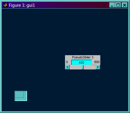
Now that we are done with the coding, start the GUI by typing gui1 in the command window. The figure window on the left will appear. As we mentioned above, the uitable and all seven uicontrols are on top of each other near the lower left corner, so we only see the last one. Likewise all three pseudo sliders are also on top of each other in the middle of the figure. Now its time to fix this problem. Type plt move in the command window to enable the mouse driven repositioning mode.

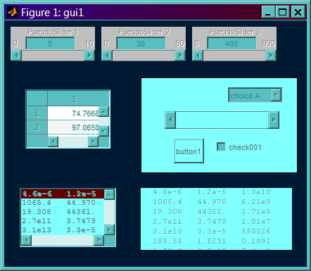
The graphical objects inside the current figure are grayed out to indicate that the repositioning mode is active. Now we can:

• left-click, hold, and drag to move an object.
• right-click, hold and drag to resizes an object.
• Double click to open an object's property inspector window.

At the stage shown here we at least have moved and resized all the objects so we can see all the individual items, none of them overlap, and they are at least close to the positions we outlined in our sketch.

I notice that the frame is too bright since I intended it to be a subtle grouping. One way to adjust this is by typing commands into the command window. After clicking on an object (in repositioning mode) a variable called "hhh" is added to the base workspace containing the object's handle. So now I can experiment with colors or other properties by typing commands such as:

set(hhh,'backgr',[1 1 2]/6,'foregr',[1 1 1]/2);.

Once I get the look I want I can copy and paste the command from the command window into the program (right before the line that saves the handles to the figure userdata):

set(h(1),'backgr',[1 1 2]/6,'foregr',[1 1 1]/2);.

Note that I changed the "hhh" to h(1) before inserting the line into the program. A second method for doing this (instead of typing the commands in the command window) is to double click on the object which will bring up the property inspector for that object. Then as you change the property values in the inspector you will immediately see the effect on the GUI. (The second method is certainly easier if you don't know the exact property names for the objects you are working with.)

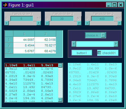
With a little more rearranging we finally get the look we are aiming for as shown here. Note that the controls are still grayed out since the repositioning mode is still active. One thing that you will notice while repositioning objects is that moving the frame also moves all the objects inside the frame. Unless you have a very old version of Matlab you may also use a uitable to allow this grouping effect. The main advantage of the uitable is that you can optionally specify a label for the grouping that will appear along the top edge. (The second example demonstrates this.)

Before exiting the program or canceling the repositioning mode click on each of the graphical objects once in the order that you created them in the program (left to right and top to bottom in the GUI). As you are clicking each item, plt will be displaying the positions of the objects in the command window. When you are done the command window will contain something similar to this:

uic: 207 .540 .500 .440 .280; % frame1
uic: 206 .680 .710 .170 .050; % choice A
uic: 205 .570 .610 .380 .060; % slider
uic: 204 .570 .520 .170 .060; % button1
uic: 203 .780 .520 .170 .060; % check001
uic: 202 .020 .050 .480 .400; % 1.79e9 8.4e-6 2.5e12
uic: 201 .540 .050 .440 .400; % 1.79e9 8.4e-6 2.5e12
sli: 401 .020 .920 .300; % PseudoSlider 1
sli: 406 .350 .920 .300; % PseudoSlider 2
sli: 411 .680 .920 .300; % PseudoSlider 3
uit: 208 .020 .500 .480 .280; % uitable

The first column is a three letter identifier for the object type. The native Matlab types - uicontrol, uitable, uipanel, axis, and text are identified as uic, uit, uip, axi, txt respectively and plt's pseudo objects are identified as sli, edi, pop, and xy. (xy refers to elements created by the cursor and plot pseudo objects.) The next column is a unique integer associated with the object. We won't need that now, but example 2 will show how that is used. The next four columns (or three columns for the pseudo sliders) specify the size and position of each object in normalized units. At the end of the line, the object type or string property of the object is included as a comment to make it clear which object the line refers to.

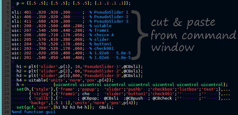
Now we are going to make the hard work we did to reposition the controls permanent. First cut and paste the 11 lines of coordinates from the command window (shown above in blue) directly into the gui1.m source code.

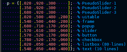
Then we fix up the 11 imported lines by deleting everything except the coordinates and comments, and adding brackets as appropriate. I've also made slight changes to the comments for clarity. I find it handy to turn on my editor's keystroke recording while fixing up the first line. Then I can replay this record to fix up the remaining ten lines by hitting the "play macro" button ten times. Most editors have this feature ... but even if you do each line manually, it's not a big deal.

Finally, in this line where we are setting the position of all seven uicontrols to the same value ... we have to change that (as shown here) so that the last seven entries of the position array are used in sequence.

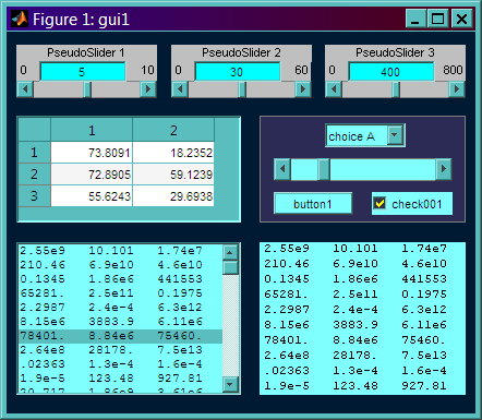
Hit save on your editor, close the gui1 figure window, type "gui1" in the command window to restart it ... and as we hoped the GUI appears just as we had organized it. Try expanding the size of the figure window and note how all the objects grow in proportion to the figure size. This is because we used normalized coordinates throughout. If you want to convert this GUI to pixel coordinates, enter repositioning mode, type set(findobj(gcf),'units','pix'), and then click on every graphics object, again in the same order as they are defined. Again, cut and paste the coordinates (which now are integer pixels) into the program as we did before. Also remove the two instances of 'units','norm' (since pixels is the default when the units aren't specified). When you run it, the GUI will at first look the same, but when you stretch the figure size, all the objects will stay exactly the same size in the same position, thus creating empty space inside the figure. Generally you will stick with either pixels or normalized coordinates, although you can mix them if it suits your purposes.

This concludes our example, although if this was a real GUI you would not likely be satisfied yet. But using the methods we just demonstrated you will be able to iterate until you are satisfied with the control types and positions.

A second example

Now that we have covered most of the basic concepts and techniques, its time to explore the true power of plt by reviewing the design of a real GUI in one of the application areas that Matlab was designed for. The application I have chosen is the display and analysis of the classical analog filters. Granted this is not a particularly novel idea as it probably has been done before in Matlab and other languages, but nonetheless it serves various educational and practical needs and there is always room to apply our own slant to the project. I'll start out with a relatively modest set of goals:

Display the magnitude frequency response for the five "classical" analog filters (Butterworth, Bessel, Chebyshev type 1 & 2, and Elliptic). The user should be able to easily select which of these filters to display, as well as allowing all of them (or any subset) to be plotted at the same time.
Interactive selection of the filter order and type (lowpass, highpass, bandpass, stopband).
Interactive selection of the number of decades to plot as well as the frequency resolution.
Both numerical entry and slider control of cutoff frequencies and pass/stop band ripple.
Cursors should be provided which allow for the easy readout of the frequency response at any point as well as delta readouts to verify stop band and pass band ripples. Peak finding should be provided as well as the ability to annotate the plot with text and markers to document features of interest.

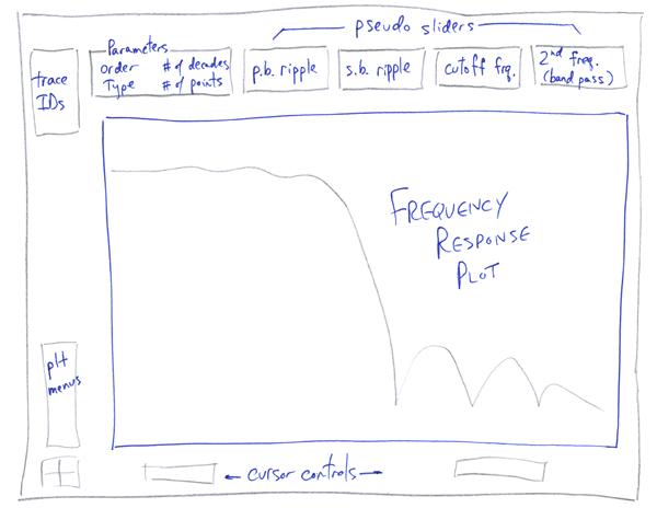
As is my habit, I start with a sketch to clarify my thoughts. I decide to use an array of four pseudo sliders along the top to control the continuously adjustable parameters (edge frequencies & ripple) The four remaining filter and display parameters are grouped to the left of the sliders inside a uipanel unimaginatively labeled "Parameters". The Trace IDs to the left of that will be named after the classical filter types and be used to select which filters to display. The plot and the cursor controls and readouts along the bottom edge are the standard ones created by the plt pseudo object.

Ok ... it's time to start writing code. First I have to come up with some first guess for the object positions, and then I define the choices for filter type and number of points to display:

function gui2()
p = {[.4 .3 .5 .5]; % plot position
[.2 .5 .1 .2]; % uipanel position: Parameters
[.2 .5 .1 .2]; % edit position: filter order
[.2 .5 .1 .2]; % popup position: filter type
[.2 .5 .1 .2]; % popup position: # of decades
[.2 .5 .1 .2]; % popup; position: # of points
[.2 .2 ]; % slider position: Passband ripple
[.2 .2 ]; % slider position: Stopband ripple
[.2 .2 ]; % slider position: Cutoff frequency
[.2 .2 ]}; % slider position: frequency 2
typ = {'low pass' 'high pass' 'band pass' 'stop band'}; pts = 100*[1 2 4 8 16];

So how good are my guesses? Look at the first screen shot below to find out. Clearly not so good. The plot is way too small compared to my sketch. All the pseudo sliders are on top of each other ... and they are near the bottom instead of near the top as shown in the sketch. Plus all the pseudo popups and edit objects are also on top of each other. But as you will see, this will not be a problem at all. In fact, it would be a waste of time to spend more than a minute coming up with the initial guess. Ok, now it is time to create the plotting pseudo object (figure, axis, cursor, grid, traces, etc):

S.tr = plt(0,zeros(1,5),'Options','LogX','Ylim',[-80 10],...
'TraceID',{'butter' 'bessel' 'cheby1' 'cheby2' 'elliptic'},...
'xy',p{1},'LabelX','radians/sec','LabelY','dB');

The 'xy' parameter is used to position the plot within the figure window (although you will soon learn that this parameter can do far more than that). The data to be plotted for all 5 traces is defined in the plt call (as it must), but notice that each trace just contains the single point (0,0). When calling plt from the command line, you almost always include the actual plot data in the argument list, however in a GUI more often than not the data supplied is just a place holder. The real data is loaded later (in the callback in this example) by using the trace handles returned by plt. Note that we save these handles in S.tr (a 1x5 array). S is the structure where we will store the handles of all the objects we define in the GUI. The remaining plt parameters should be reasonably self explanatory. Next we create the uipanel and the four pseudo objects that we will put inside it:

uipanel('units','norm','title','Parameters','backgr',get(gcf,'color'),...
'pos',p{2} ,'high',[.4 .4 .4],'foregr',[.4 .4 .4]);
S.n = plt('edit', p{3} ,[6 1 25],'callbk',@clb,'label',{'Order:' .05});
S.typ = plt('pop', p{4} ,typ,'callbk',@clb,'swap');
S.dec = plt('pop', p{5} ,1:5,'callbk',@clb,'index',3,'label','Decades:');
S.pts = plt('pop', p{6} ,pts,'callbk',@clb,'index',2,'label','Points:');

For the uipanel, I set the background color to be the same as the figure color to give it a transparent look. For both the border outline and the text label of the uipanel I used light grey (rgb = .4 .4 .4). The uipanel wasn't invented yet for Matlab 6, so there is an alternate version of gui2.m called gui2v6.m in the demo folder where this uipanel was replaced by an axis. Note that the tag property of the axis was set to 'frame'. This is to tell plt that moving the axis in repositioning mode should also move all the objects inside it (even objects not children of the axis).

The [6 1 25] parameter of the pseudo edit object means that its initial value will be six with min/max limits of 1 and 25. The string 'Order' is used as a label for the edit object, and the ".05" tells it how much space to allocate for the label (in normalized coordinates). The parameters for the three pseudo popup objects are probably more obvious, but if not, consult the Pseudo objects page. Next we create the pseudo sliders:

S.Rp = plt('slider',p{7} ,[ 2 .01 9],'Passband ripple', @clb);
S.Rs = plt('slider',p{8} ,[ 40 10 120],'Stopband ripple', @clb);
S.Wn = plt('slider',p{9} ,[.02 .001 1],'Cutoff frequency',@clb,5,'%4.3f 6 2');
S.Wm = plt('slider',p{10},[.2 .001 1],'frequency 2', @clb,5,'%4.3f 6 2');

The [2 .01 9] on the first slider has the same meaning as the similar pseudo edit parameter mentioned above - i.e. 2 is the initial value with min/max limits of .01 and 9. The @clb specifies the callback function. (Note that same callback function is used for all the controls.) The "5" after the callback function indicates that the slider will move logarithmically (so for example the slider will move the same number of pixels going from .01 to .1 as it does when changing from .1 to 1. The final parameter '%4.3f 6 2' is shorthand for '%4.3f %6v %2v' and specifies the display format for the min value, current value, and max value respectively. Now we have just a few more lines left to complete the gui2.m function:

set(gcf,'user',S);
clb;
% end function gui2

The first line saves the handle structure in the figure user data where the callback function can easily retrieve it. The next line (the last of the gui2 function) executes the callback function to initialize the display to agree with the initial values of the controls. After just 17 lines of code, we're finished writing the main line function, plus 10 more lines for our initial guess for the control positions. But now the real work begins - the callback function that makes the GUI come alive:

function clb() % callback function for all objects;
S = get(gcf,'user'); % get handle structure
ty = plt('pop',S.typ);    % get filter type index
t = {'low' 'high' 'bandpass' 'stop'}; t = t{ty}; % get filter type name
N = plt('edit',S.n); % get filter order
dec = plt('pop',S.dec); % get number of decades to plot
pts = str2num(get(S.pts,'string')); % get # of points to plot
X = logspace(-dec,0,pts); W = X*1i; % X-axis data (radians/sec)

First we pick up the filter parameters that are inside the uipanel (filter type, order, number of points, number of decades). You might wonder why I seem to repeat myself by defining the filter types again since it would seem more logical to simply get the filter type with get(S.typ,'string'). That command would retrieve one of the following strings: {'low pass' 'high pass' 'band pass' 'stop band'}, but the strings accepted by the Matlab filter functions are slightly different: {'low' 'high' 'bandpass' 'stop'}. It would have been much easier just to use the strings that Matlab requires for the popup control, but I was too picky about the look of the popup control to use those somewhat inconsistent strings. Finally the logspace command generates the requested number of points logarithmically spaced between .001 and 1 (for the 3 decades example). W is this same vector on the imaginary axis, which is used with polyval to compute the frequency response function.

Wn = plt('slider',S.Wn);    % get filter freq
Rp = plt('slider',S.Rp);    % get passband ripple
Rs = plt('slider',S.Rs); Rs2 = max(Rp+.1,Rs); % get stopband ripple (must be > passband)
if ty>2 Wn = [Wn plt('slider',S.Wm)]; % get frequency 2
plt('slider',S.Wm,'visON'); % make frequency 2 slider visible
else plt('slider',S.Wm,'visOFF');    % make frequency 2 slider invisible
end;

Next we pick up the filter parameters from the four pseudo sliders. Note that for the last two filter types (bandpass and stopband) we need the second frequency slider ("frequency 2") and so this slider is only visible when one of those filter types is selected.

[B,A] = butter(N,Wn,t,'s'); H{1} = polyval(B,W)./polyval(A,W);
[B,A] = besself(N,Wn(1)); H{2} = polyval(B,W)./polyval(A,W);
[B,A] = cheby1(N,Rp,Wn,t,'s'); H{3} = polyval(B,W)./polyval(A,W);
[B,A] = cheby2(N,Rs,Wn,t,'s'); H{4} = polyval(B,W)./polyval(A,W);
[B,A] = ellip(N,Rp,Rs2,Wn,t,'s'); H{5} = polyval(B,W)./polyval(A,W);
if ty~=1 H{2}=H{2}+NaN; end; % bessel filter only applicable for low pass

Then we use the Matlab classical filter functions to compute the numerator and denominator s-plane polynomials (B,A) and compute the frequency response using polyval. Although it would have been slightly shorter to use freqs() instead of polyval(), I didn't do that since freqs is part of a toolbox that some users will not have. If a filter type other than low pass is selected, the last line changes the Bessel transfer function to "NaN" so that the trace will not appear on the plot. (The Bessel filter is only defined for low pass.)

for k=1:5 set(S.tr(k),'x',X,'y',20*log10(abs(H{k}))); end; % set trace data
plt('cursor',-1,'xlim',X([1 end])); % set Xaxis limits
% end function clb

Then we use the absolute value function to compute the magnitude of the frequency response, and convert to dB (20*log10) before placing the result in the y-axis property of the 5 traces. Finally to set the x-axis limits in case they have changed (which happens when the callback is in response to the "number of decades" control).

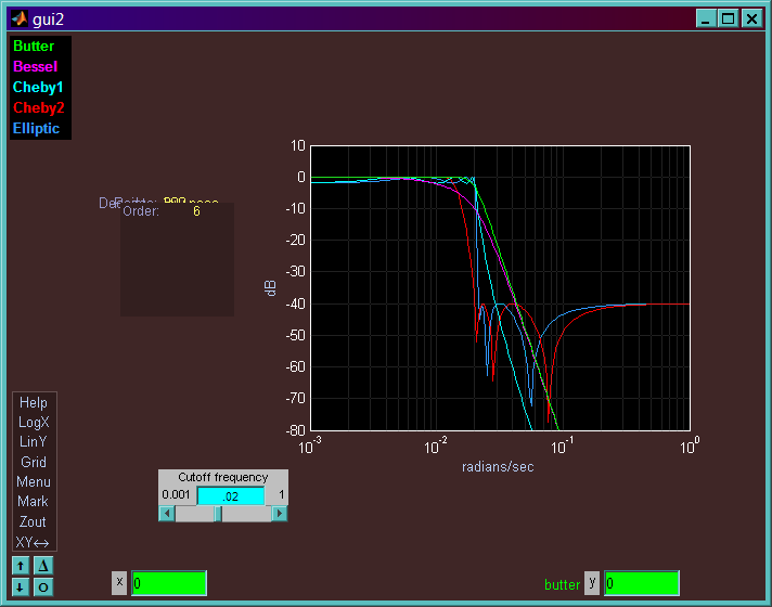
Finally we are done with the initial coding and we can try it out. Typing "gui2" to start the program brings up this figure. Although all the controls are there as promised, they are not anywhere close to being in the right place, but it will take only a few minutes to fix this. Begin by entering "repositioning mode" by right-clicking on the delta button (or if you prefer, by typing plt move.) Then as I described in the previous example, use a left click and drag to move the objects around and a right click and drag to resize them.

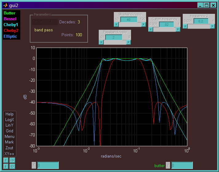
I still don't have the final positioning, but it's close. The uipanel contains the controls it should and the other objects are also at least in the vicinity of where they should be. Note that once objects are placed inside the uipanel, moving the uipanel will also move all the objects inside it. After a few more tweaks, we will have at least our first cut positioning. Before closing this figure it is important to remember to left-click once on every object, in the order that they were created in our program. As we are doing this, the text below will appear in the command window:

xy: 1 .130 .105 .840 .760; % axes
uip: 213 .100 .885 .240 .110; % uipanel
edi: 211 .165 .935 .040 .030; % 6
pop: 102 .110 .710 .100 .200; % band pass
pop: 103 .310 .750 .020 .200; % 3
pop: 104 .287 .710 .054 .200; % 200
sli: 401 .350 .946 .150 ; % Passband ripple
sli: 406 .510 .946 .150 ; % Stopband ripple
sli: 411 .670 .946 .150 ; % Cutoff frequency
sli: 416 .830 .946 .150 ; % frequency 2

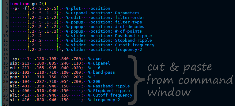
Then as before, we copy and paste those lines into the source code as shown here.

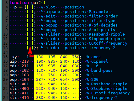
We could fix up the brackets and comments line by line as we did in the previous example, however since my editor has a column select mode (as pretty much every programmers editor does) I find it easier to block delete the old coordinates (our rough first guess) and then do a block move (as shown by the red arrow) the new coordinates into the blank array.

We're done with the repositioning step, so we hit save in our editor, restart the application and we should see a figure similar to the one below.

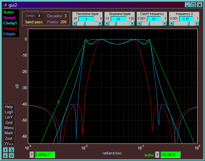
Now we can play with all the controls and make sure everything is behaving as we imagined. Not bad considering we've written a non-trivial GUI applications involving non-trivial filter computations by writing only 51 lines of code. (Fewer if you don't count the automatically generated table of numbers that specify the object positions.) It's the power of the pseudo objects that allows the program to be written so quickly and concisely.

Of course what nearly always happens the first time you get to experiment with your GUI is that you will have some new ideas:

Perhaps this isn't the most convenient set of controls. Would it be more useful to have fewer controls, more controls, ... or just different controls?
Even if the controls seem appropriate, perhaps it would be more esthetically pleasing to rearrange and resize them?
Do we have features that we don't really need? Or can we add useful features without making the GUI too complicated?
Can we rearrange or refactor the code to make it easier to understand and adapt?

Indeed when I got to this stage of testing the application I did have a few enhancement ideas:

I was curious (mostly for the elliptic filter) how the width of the transition band (the space between the passband and the stopband) varied as the filter order changed as well as the four slider parameters. Could I define such a measure, figure out how to compute it and find a place on the GUI to display it?
My second idea was to allow the user to control at least some aspect of the color choices used in the application. Actually I don't think such a simple application like this really needs this flexibility, but my ulterior motive was to showcase the ColorPick pseudo object and how easy it is to add to your GUI and how easy it is to select the color you find most pleasing for any display element.
What does the phase response of these filters look like? Could I add a display of the phase response without cluttering up the plot or obscuring the magnitude response (which is still the primary interest).
It would be nice if whenever we made a change to the figure size/position or the color selection, that these changes would be recorded so that the application looks the same the next time it is restarted. While we are at it, we might as well remember the state of the eight filter parameters (shown above the plot) so that on start up, the figure looks identical to the way it was when it was shut down.
Finally lets add a very brief set of help messages to allow a new user of the program to get started without having to consult any help files or manuals. The most important consideration should be that the help messages are not distracting in any way to the user who is already familiar with the help information presented.

These enhancements turned out to be fairly easy to implement. You can look at the final code which includes these enhancements (gui2.m in the plt\demo folder) or read on to find out more about the process.

1.) Adding a multi-line text string (elliptic transition ratio)

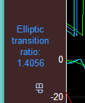
For a low pass filter, I characterized the transition width in terms of the ratio of these two frequencies:
• The frequency where the stop band spec is first achieved
• divided by the last frequency where the passband spec is still achieved
For a high pass filter, the ratio is:
• The frequency where the pass band spec is first achieved
• divided by the last frequency where the stopband spec is still achieved

I added an 11th line to the position array at the beginning of the program, to define the location for the new text object. Initially it was just a wild guess as usual which was refined using the repositioning mode:

[-.09 .650 ]; % text position: elliptic transition ratio

The text object was created with this line (added after the slider definitions):

S.etr = text(0,0,'','pos',p{11},'units','norm','horiz','center','color',[.2 .6 1]);

Note that the string to display was set to null, because the actual string to display will be set in the callback function as follows:

h = find(get(S.tr(5),'y') < -Rs2); % find indices where the stopband spec is satisfied
if isempty(h) h = 0; % stopband specification not achieved
elseif (ty-2)*(ty-3) h = X(h(1))/Wn(1); % computation for lowpass & stopband filters
else h = find(diff([h inf])>1); h = Wn(1)/X(h(1)); % computation for highpass & passband filters
end;
set(S.etr,'string',prin('Elliptic ~, transition ~, ratio: ~, %5v',h));

This last line takes advantage of prin's cell array delimiter feature to create the multi-line string used to display the elliptic transition ratio in the small space available on the left side of the plot. To learn more about prin and the %v format used here, check out the Auxiliary functions.

2.) Selecting colors

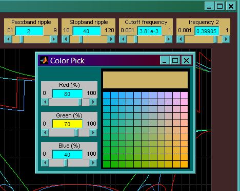
This was one of the simplest of the five enhancements requiring just the three extra lines shown below. I decided to enable color adjustment of just the pseudo sliders (the most prominent controls), although it would be easy to extend this to other graphic elements. In this figure I have changed the background color of the sliders from its default gray to orange. I encourage you to play around with this ColorPick figure. (Just right-click on any of gui2's pseudo sliders to bring up ColorPick.) If you have ever dealt with the frustrations of assigning screen colors, I think you will be pleasantly surprised about how easy it can be. Also you can read about the ColorPick details near the bottom of this page: Pseudo objects

The first line (below) gets puts the handles of all the objects associated with pseudo sliders into "h". Then the 5th element of each slider is removed, since that is the edit box portion which generally is set to a contrasting color. The second line assigns the ColorPick object as the buttondown function (the action associated with right clicking on the pseudo slider). The third line is necessary to tell ColorPick which property of these objects should be adjusted when a new color is chosen (the background color in this example).

h = getappdata(gcf,'sli'); h(5:5:end) = [];
set(h,'buttondown','plt ColorPick;');
for k = 1:length(h) setappdata(h(k),'m',{'backgr' h}); end;

3.) Linking traces (adding the phase display)

To add the phase display, the most important change is in the callback function. Before we set trace data for 5 traces, but now we must set trace data for 10 traces (the first five for magnitude and the last five for phase):

for k=1:5 % set trace data
set(S.tr([k k+5]),'x',X,{'y'},{20*log10(abs(H{k})); angle(H{k})*180/pi});
end;

Then we just need to increase the data array defining the traces in the plt call from 5 to 10, specify that the last 5 traces should be on the right hand axis ... and we would be done. However then we would need 10 TraceIDs up there as well. I didn't want that because then to enable or disable the trace for the cheby1 filter (for example), I would have to click on two TraceID tags. Not so convenient. Also by default, ten different colors would be chosen for the ten traces. This would make it more difficult to tell which phase trace was associated with which magnitude trace. Both these problems are fixable of course:

c = [0 1 0; 1 0 1; 0 1 1; 1 0 0; .2 .6 1]; % trace colors
lbl = {'dB' [blanks(70) 'Phase \circ']}; % y-axis labels: {left, right}

The first line above defines the trace colors that also happen to be the default colors normally used for the first five traces. Only we are going to use them below for both the first five traces as well as for the last five traces. The next line defines the y-axis labels for both the left axis (magnitude response in dB) and for the right axis (phase response in degrees). Note the Tex command "\circ" in the right axis which inserts a small circle (the degree symbol) into the label. The 70 blanks that are inserted in front of the right hand label is used to push the label up towards the top of the display where the phase information will be plotted. And finally we have to fix up the main plt call:

S.tr = plt(0,zeros(1,10),'Right',6:10,'Options','LogX',...
'DualCur',-5,'TraceID',{'butter' 'bessel', 'cheby1' 'cheby2' 'elliptic'},...
'Ylim',{[-90 60] [-1000 200]},'LabelX','radians/sec','LabelY',lbl,...
'TIDcback','t=plt("show"); t=t(find(t<6)); plt("show",[t t+5]);',...
'xy',p{1},'TraceC',[c;c],'+Ytick',-140:20:0,'-Ytick',[-180 0 180]);

Some of the parameter changes in the plt call were already mentioned, but some others merit mention:

The 'DualCur' parameter with minus five as an argument tells plt that the second trace number that should be cursored is offset from the first one by five. This means for example, if you click on trace 2, not only will a cursor appear on trace 2, but trace 7 will also have a cursor. (And each cursor will have a separate readout edit box as well.)
The 'Ylim' parameter now includes two sets of y limits. As with the 'LabelY' command, the first entry is for the left axis and the second is for the right axis. The limits have been chosen to position the magnitude response on the lower portion of the graph and the phase response on the upper portion.
The '+Ytick' and '-Ytick' parameters specify the tick marks to be used on the left and right hand axis (respectively). We don't technically need these parameters, but it looks better to include tick marks only in the area where the data can be located.
The addition of the 'TIDcback' parameter is perhaps the most interesting. This defines a callback function that is executed every time you click on any one of the TraceID text strings. Here, the plt('show') function (see "Single argument actions" near the end of this page) is used to enable only those phase traces that correspond to magnitude traces that are also enabled.

4.) Saving/restoring the GUI state using a configuration file

Before the call to plt, let's choose a file name and path for saving the configuration data: S.cfg = [which(mfilename) 'at'];

Next let's add a new function, called cfg which saves the current configuration to the file:

function cfg()
S = get(gcf,'user'); sli = findobj(gcf,'style','slider');
cf = { plt('edit',S.n);    plt('pop',S.typ);
   plt('pop',S.dec); plt('pop',S.pts);
   plt('slider',S.Rp);   plt('slider',S.Rs);
   plt('slider',S.Wn);   plt('slider',S.Wm);
   get(sli(1),'backgr'); get(gcf,'pos') };
save(S.cfg,'cf');

Then right before we initialize the plot, we load the configuration file if it exists and set the GUI elements to agree with the data in the file:

if exist(S.cfg) load(S.cfg);
plt('edit',S.n,'value', cf{1}); plt('pop',S.typ,'index',cf{2});
plt('pop',S.pts,'index',cf{3}); plt('pop',S.dec,'index',cf{4});
plt('slider',S.Rp,'set',cf{5}); plt('slider',S.Rs,'set',cf{6});
plt('slider',S.Wn,'set',cf{7}); plt('slider',S.Wm,'set',cf{8});
set(h,'background', cf{9}); set(gcf,'position', cf{10});
end;

And finally we add this parameter to the plt call:

'closeReq',@cfg

This instructs plt to call the function that saves the configuration data when the user closes the figure window to exit the application.

5.) Adding temporary user help message

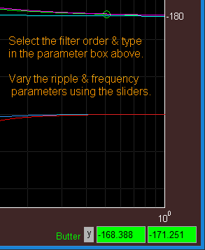
The HelpText pseudo object is ideal for this task since it provides a mechanism for removing the messages once you start using the program. To define the help text and make it visible on the screen, these three lines were added to the end of the main gui2 routine:

htxt = {'Select the filter order & type' ...
'in the parameter box above.' '' ...
'Vary the ripple & frequency' ...
'parameters using the sliders.' .6+.62i};
plt('HelpText','on',htxt); % show help text

Note that we have defined a help message consisting of five lines of text (with the middle line is blank). The complex number at the end specifies the position relative to the main axis where we want the help text to appear. The real part specifies the horizontal position and the imaginary part specifies the vertical position (in normalized units). And lastly, this line was added to the and of the callback function (clb):

plt('HelpText','off');

That line insures that as soon as the user starts doing anything with the program, the HelpText will disappear insuring that it does not become a distraction.

This concludes our discussion of the gui2 example. Although it might seem like coding this example was a lot of work, only about 85 lines of code were needed to implement a fairly complex set of display and computational requirements. GUI programming is notorious for its complexity, and I believe that if you tried to implement a this application in other programming languages you would be looking at a far larger effort with source code running into the many hundreds of lines. I would like to be able to report how long the program would be in Matlab using GUIDE (without using plt), so I would be thrilled if one of the guide experts out there would take up this challenge by implementing the original five goals of gui2 as well as the five enhancements. If you manage to do this, I would gladly include your GUI (with credit of course) to contrast the Guide programming style with the one I present here.

To further your education of GUI programming with plt, I especially recommend reviewing the pltsq.m application if you are interested in moving plots (i.e. real-time updating). Also the curves.m, editz.m, pltmap.m, and winplt.m applications are worth reviewing since they each have a fairly rich GUI design with lots of opportunities for using various plt features in interesting ways.

SnapTo resolution

You may have noticed that in repositioning mode, the objects when dragged don't move or resize smoothly, but rather move in steps of a fixed size. This makes it easier to align related objects and generally gives a more pleasing result. The default grid size is 100 by 100 which means that there are 100 useable positions inside the figure in both the x and y directions. This also means that if you are using normalized coordinates the third decimal place for all position vector elements will be zero.

There are three ways to bring up the SnapTo figure shown below:

Type plt move res in the command window. (This is the only method if you are not using a plot pseudo object).
First left-click on the delta button, followed by a right click on the same button.
It's easy to forget the sequence for method two, so you can also go to the plt menu in the menu bar. There you will see the option "Reposition grid size" which will bring up the SnapTo figure.

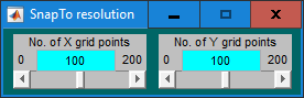
The default resolution is usually enough, but if you want finer control, move one or both of these sliders to the right edge (i.e. 200). This is nearly always enough, although if you like you can type in a number bigger than 200 into either edit box. Or you can move the slider all the way to the left (i.e. zero) which disables the snap-to feature altogether.

previous page start next page